
Unlock faster data processing for Machine Learning: reducing pivoting time from hours to minutes
Training Machine Learning models on big data isn’t just about fitting the model itself — it’s about efficiency at every stage
of the process. While much attention is given to optimizing model training itself, the earlier phases can be just as, if not more,
critical to the overall performance. In this article, we take a deep dive into what happens before we actually invoke model.fit(),
focusing on the data pivoting stage. We are taking you on a journey through various pivoting solutions, exploring both pitfalls and interesting optimizations.
The goal is simple: make this process highly efficient — in terms of processing time and memory usage. So, buckle up!
What do we do and why to care about data pivoting #
At Allegro, we work on a variety of Machine Learning solutions. Given Allegro’s scale as one of the largest e-commerce platforms in Europe, the data volume we handle is usually massive. In this article, we’ll explore specific areas of the AllegroPay ML Platform, where we conduct and support various processes related to credit risk and marketing models within the payments domain.
At a high level, the process consists of the following steps:
- Gathering and storing the data.
- Data cleaning.
- (optional) Exploratory data analysis.
- Feature engineering and feature selection.
- Training, evaluating, deploying and monitoring of a model.
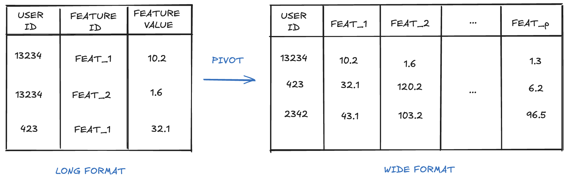
During this journey, let’s focus on feature engineering aspects (step 4). If you’ve ever trained an ML model with any standard ML library (like scikit-learn), you know that, before training, models usually expect a dataframe in a wide format, where each feature has its own column. For simplicity, let’s assume in our case an observation is a single user, so wide-format columns could be defined as: USER_ID, FEATURE_1_VALUE, FEATURE_2_VALUE, …, FEATURE_P_VALUE.
At AllegroPay ML Platform, we use Snowflake warehouse for data processing purposes. The entry point to feature engineering step is a Snowflake table with features stored in a long format. In a long-format table, each row represents a value of a given feature for a given observation. The columns of the long format table are then defined as: USER_ID, FEATURE_ID, FEATURE_VALUE. It means that before training, we need to transform the data from long to wide format — we need to PIVOT the data.
Now, you might be wondering: if ML models require wide format, why to store features in a long format? ;) There are two reasons. Firstly, storing data in a long format allows us to add new features easily. There’s no need to change table schemas to add columns representing new features — we simply insert new rows. The second reason is the architecture of Snowflake. Wide-format storage would quickly incur a large number of columns, which is not optimal for Snowflake queries.
Now we know that we need to pivot the data and we understand why. Let’s do it then!
The standard solution and the problem #
Data pivoting may seem like a standard problem, so a mature warehouse provider like Snowflake has to have an out-of-the-box solution for that. Indeed,
there is a SNOWFLAKE PIVOT function, ready to be used. The problem is that, for our use case, it works really slowly, even for medium-sized data
volumes. For the benchmark tests of all the following solutions, let’s consider an exemplary long-format data sample containing a few thousand features,
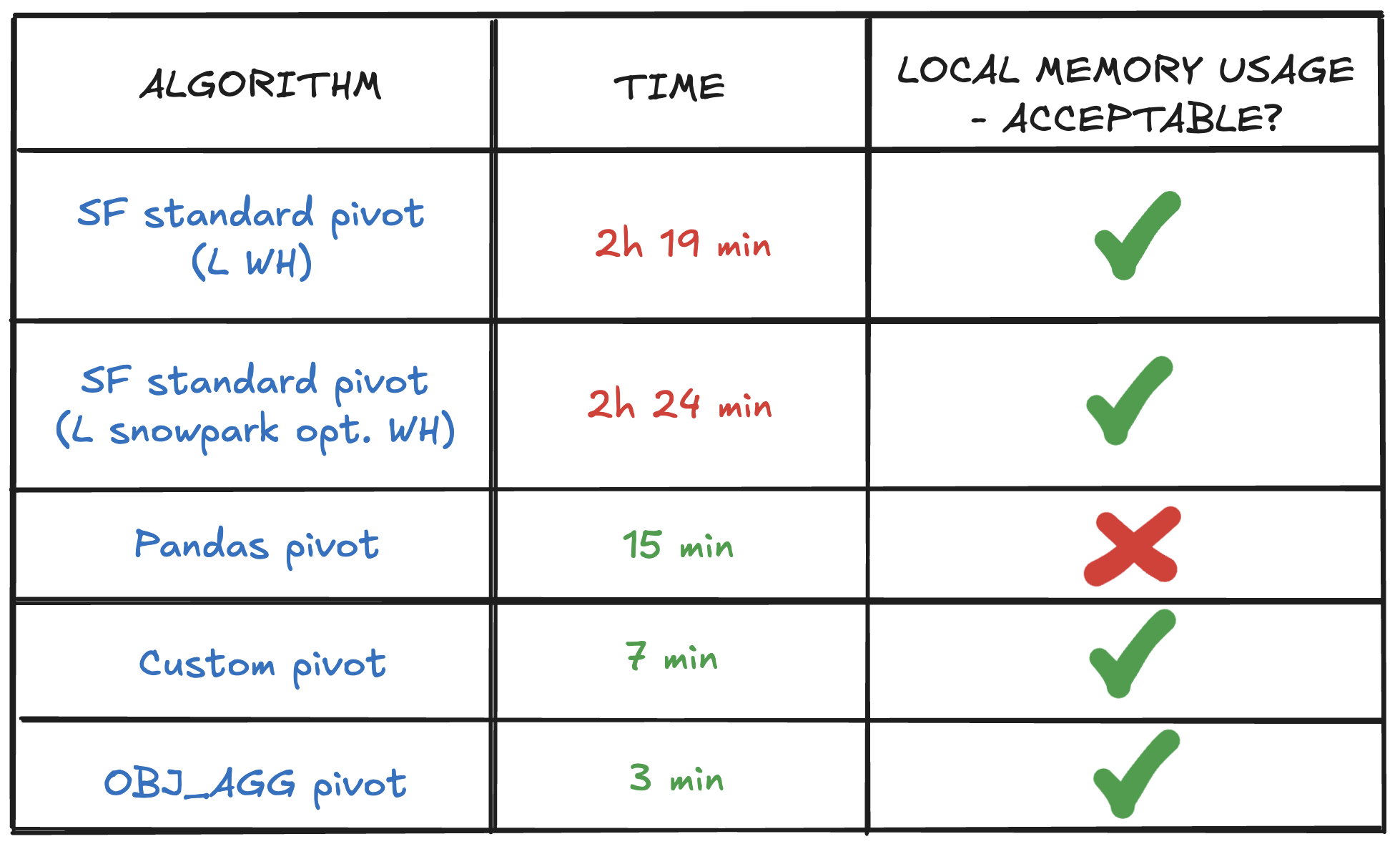
resulting in hundreds of millions of rows in a long-format table. Transforming it with SNOWFLAKE PIVOT takes 2 hours and 19 minutes, so is unacceptable — real
samples used for training tend to have 20x more observations and 10x features. The reason for that is probably the fact that SNOWFLAKE PIVOT is designed
to handle all pivoting variants generically and our case is in a sense simplified (we, for instance, do not perform aggregations).
First guess: let’s change the warehouse type #
At the core of Snowflake computing are virtual warehouses — clusters of compute resources that provide CPU, memory, and temporary storage. Warehouses enable queries and calculations on data stored in Snowflake tables. Snowflake offers multiple types of warehouses, each differing in computing power. For every operation, we can assign a warehouse that best matches our performance needs.
While working with Snowflake, the first, no-brainer way to speed things up is often switching to a more powerful warehouse and observing what happens. However, usually, this is not the solution you want to apply permanently, as it can lead to a sudden increase in costs ;). As in our training process we interact with Snowflake via Python Snowpark (a set of libraries and code execution environment for interacting directly with Snowflake data via Python API, modeled after PySpark), we went for a special type of computing — Snowpark-optimized warehouse. This warehouse type provides additional memory for processing and can potentially accelerate Snowpark calculations.
Nonetheless, changing the warehouse to Snowpark-optimized didn’t help — in our tests, it worked similar to a standard warehouse. For the benchmark sample, the pivoting time with a Snowpark-optimized warehouse was 2 hours and 24 minutes.
Back to the good old Pandas? #
Years go by, yet the Data Science community’s attachment to Pandas remains strong. Pandas provides built-in pivoting functionalities, so why not use it? If you’ve worked with large datasets, you probably already know the answer.
In such processes, we need to consider not only the execution time but also the memory usage. Simplifying: to perform pivoting, pandas is going to load the entire dataset into memory. While it isn’t an issue for small samples (our relatively small benchmark took around 15 minutes), in big data scenarios, it would require an enormous amount of RAM. It leads to impractical costs, making pandas an unfeasible choice for large-scale processing.
Let’s do it on our own — custom pivoting #
As none of the out-of-the-box solutions worked for us, we decided to rethink the process and design a solution directly addressing our requirements: time and memory efficiency. By analyzing our data patterns, we arrived at the following key insights:
- Our data does not contain multiple feature values for a single (USER_ID, FEATURE_ID) pair => we do not need to perform aggregations during pivoting.
- We know the number of features and their identifiers => we can process features separately and apply parallelism — we know how many processes we need.
- Each observation contains the same number of features => we can calculate the number of observations based on just one feature.
- In addition to knowing the number of features and observations, we also have information on data types => we can estimate the memory usage.
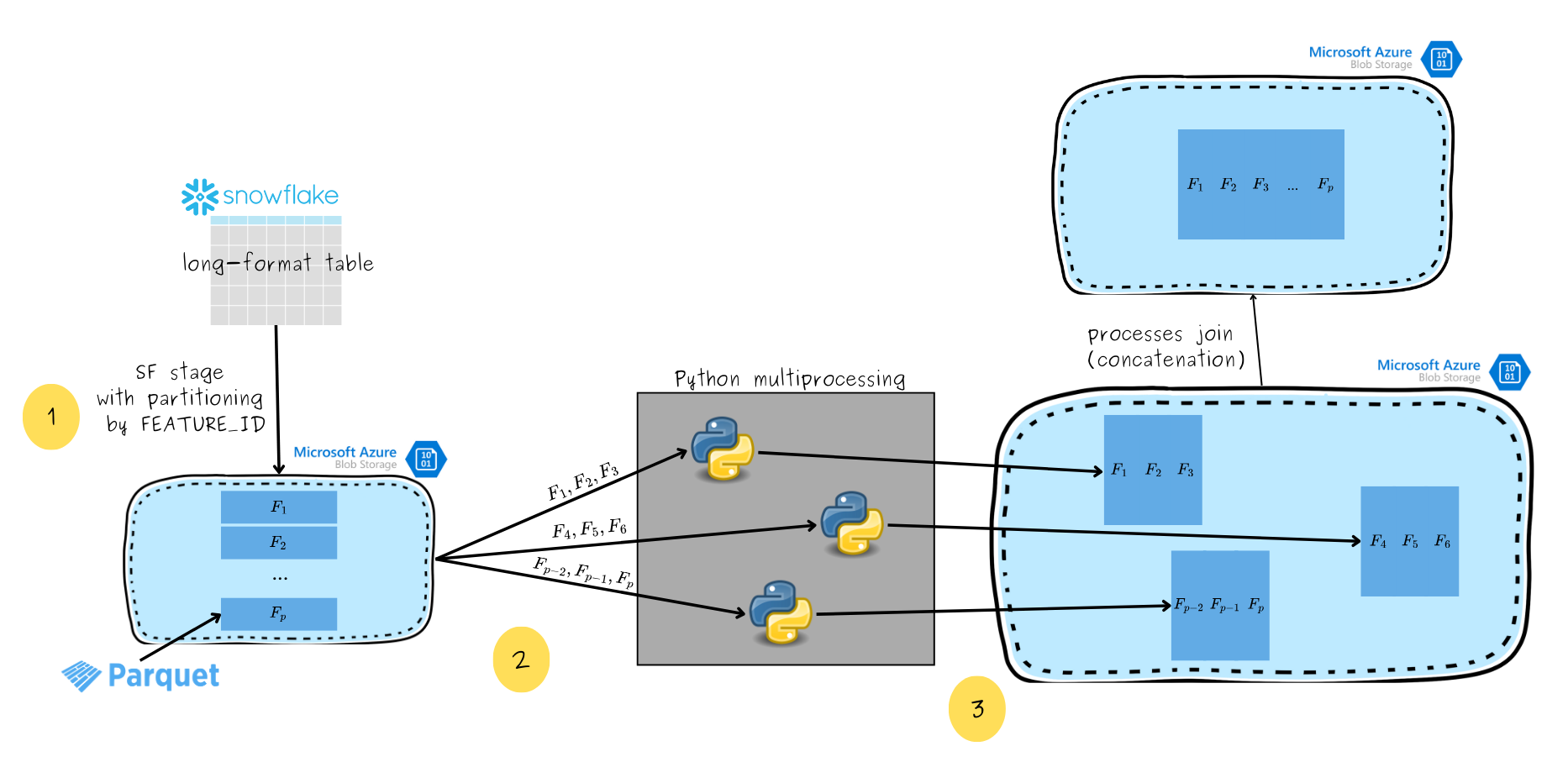
Considering the potential for parallelism and granular memory control, we adopted the following approach (see the picture below):
- We start with a long-format Snowflake table, that is partitioned by FEATURE_ID and stored in Azure Blob in separate parquet files. As a result, each parquet file contains data from only one feature.
- Then, each process queries the dataset to retrieve a batch of features it is responsible for. In this article, a batch of features refers to feature values for all entities (USER_IDs) and some set of features. For example, one batch of features could be composed of features F1, F2 and F3, as showed in the picture below. Only selected features (the ones from a specific batch) are loaded into memory.
- Pivoted batch is saved back to Azure Blob, again as a parquet file. We end up with a set of parquet files, each containing a set of wide-format features. The last step is to join the results of different processes — concatenate the files into one, wide-format parqet file.
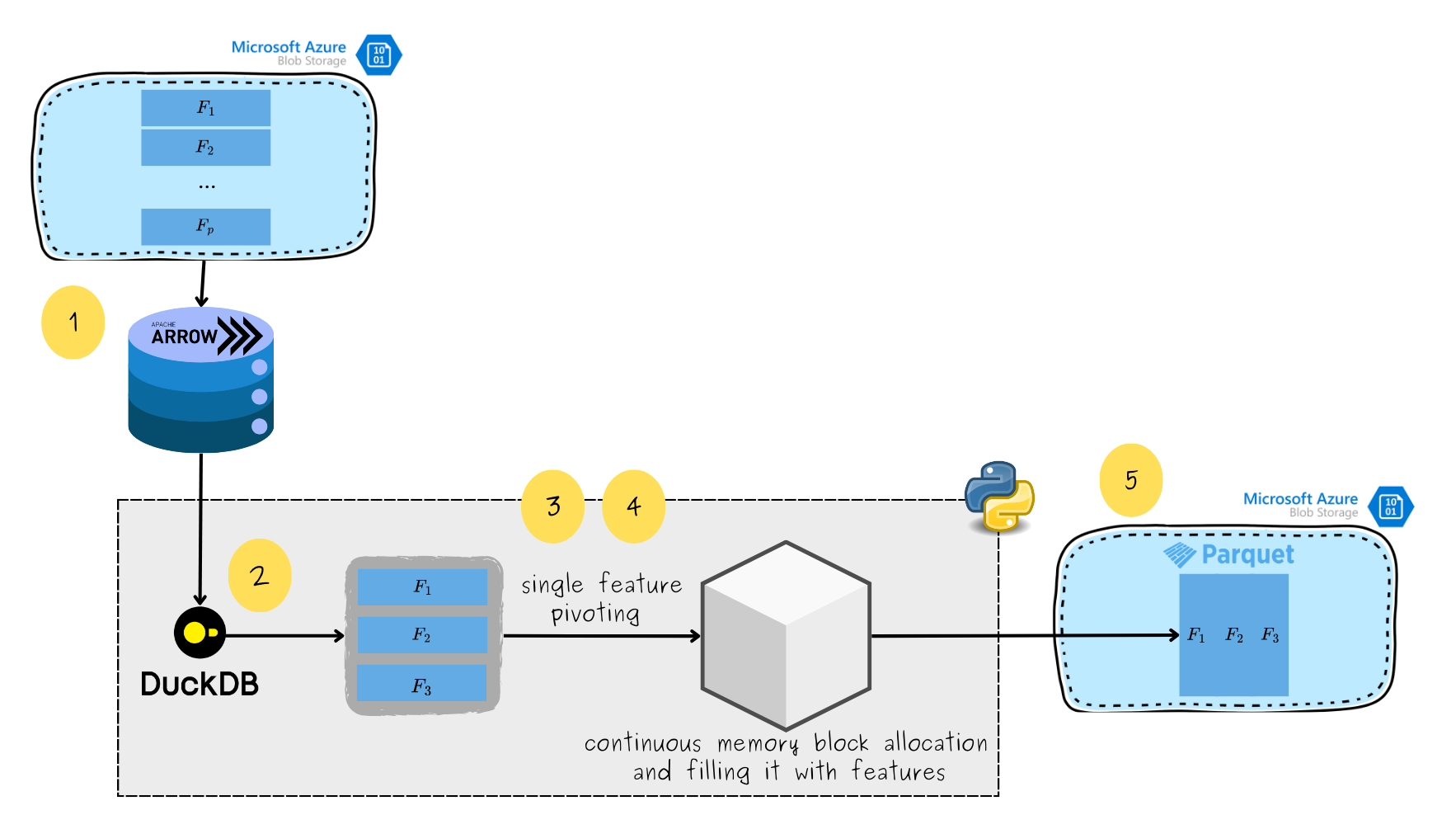
Let’s have a look at what each process does (see the picture below):
- We first treat the partitioned dataset as a PyArrow dataset, leveraging the efficiency of the Apache Arrow format. Apache Arrow allows us to efficiently query subsequent columns without loading lots of data into memory at once.
- Then, each process queries the dataset to retrieve a batch of features it is responsible for. It is performed with DuckDB which allows us to load only the required features into memory, rather than the entire dataset.
- The process knows how many features and observations it handles and what are the data types. It means it can calculate its exact memory needs. Based on this, the process allocates a continuous memory block, which will later be filled with features.
- The process first fills the memory block with observation IDs (USER_ID), followed by pivoted features from the batch, stored as subsequent columns.
- Finally, the entire wide-format memory block is saved as a parquet file in Azure Blob.
An important question is: how do we adjust the number of parallel processes and the memory quotas per process? An initial guess for the number of processes could be the number of CPU cores available. For instance, I tested this approach on my personal Mac with 12 cores using the benchmark sample. It turns out that the optimal number of processes is actually much higher — around 32 processes to achieve the shortest pivoting time (plot below). After giving it some thought, the reason is quite clear: our processes rely heavily on IO operations (in this case, interacting with Azure Blob to download and save data). While one process is blocked during an IO operation (not using the CPU), another process can be scheduled by the operating system to utilize the available CPU core. In our tests, the effective heuristic was to use 2-3 times the number of available CPU cores for the number of processes. As for the memory quota per process, it can be calculated by dividing the total available memory by the number of processes.
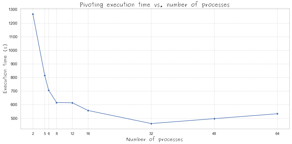
As you can see in the picture above, this solution reduces the pivoting time to around 7 minutes. Moreover, it fully controls the memory used, so I was able to achieve this pivoting time on my personal Mac with 32 GB RAM.
Step back — seeking a Snowflake solution #
For now, we have an acceptable solution, satisfying both time and memory requirements. It gives a full control over the memory management,
but it comes with a cost — we have to transfer the data out of Snowflake at the pivoting stage. While in cases the after-pivot processing
is done on a different compute (Virtual Machine, local computer), it is not a problem, since we have to do it anyway. On the other hand, if
we still want to process the data with Snowflake warehouses, it would be beneficial not to move it back and forth.
That’s why we delved deeper into Snowflake’s capabilities. With guidance from Snowflake experts, we came across a solution that, though unconventional,
turned out to be advantageous: the object_agg function.
Object aggregation in Snowflake is a tool for processing semi-structured data, and it’s default use isn’t data pivoting.
object_agg operates on groups of rows, returning for each group a single OBJECT, containing key:value pairs.
In our case, we utilize it for pivoting in the following manner (see the schema below):
- We group the data by USER_ID.
- Then, for each group we apply the
object_aggfunction, which, for each user, results in an object withkey:valuepairs, wherekeyis the feature ID andvalueis the feature value of that feature for a given user. - By appropriately selecting from the resulting OBJECTs, we get the wide-format data, which is then saved in a Snowflake table.

Let’s see how this solution works in Snowpark code. First, we need to include all necessary imports, retrieve a Snowflake session and prepare some mock data:
from snowflake.snowpark.functions import col, object_agg
from snowflake.snowpark import Session
from snowflake.snowpark.types import StructType, StructField, \
    IntegerType, StringType, FloatType
from snowflake.snowpark.context import get_active_session

session = get_active_session()

schema = StructType([
    StructField("USER_ID", IntegerType()),
    StructField("FEATURE_ID", StringType()),
    StructField("FEATURE_VALUE", FloatType())
])

data = [
    (1, 'F1', 2.4),
    (1, 'F2', 3.1),
    (2, 'F1', 5.3),
    (2, 'F2', 8.8)
]

long_format_data = session.create_dataframe(data, schema=schema)
Then, let’s perform object aggregation:
obj_aggregated_data = long_format_data.group_by("USER_ID") \
    .agg(object_agg("FEATURE_ID", "FEATURE_VALUE").alias("result"))
obj_aggregated_data looks like this:
obj_aggregated_data.show()
+---------+------------------------+
| USER_ID |        result          |
+---------+------------------------+
|    1    | {"F1": 2.4, "F2": 3.1} |
|    2    | {"F1": 5.3, "F2": 8.8} |
+---------+------------------------+
And finally, select the features from the resulting OBJECTs to obtain a pivoted dataframe:
cols_to_select = ["USER_ID"] + [
    col("result")[key].cast("float").alias(key) for key in ["F1", "F2"]
]

wide_format_data = obj_aggregated_data.select(*cols_to_select)
Our final, pivoted dataframe is exactly what we need:
wide_format_data.show()
+---------+--------+--------+
| USER_ID |   F1   |   F2   |
+---------+--------+--------+
|    1    |   2.4  |   3.1  |
|    2    |   5.3  |   8.8  |
+---------+--------+--------+
This approach turned out to be the most effective one, reducing the pivoting time to around 3 minutes, all while keeping the data within Snowflake!
Conclusion #
The pivoting journey ends up with two satisfiable solutions: one working fully locally — outside of Snowflake (custom pivoting),
and the other one leveraging Snowflake capabilities (object_agg pivoting).
The advantage of the custom approach is that it provides full control over the memory management, enabling efficient pivoting of large data
even on personal computers with limited RAM. In turn, the object_agg solution is the most time-efficient and does not require
data transfer outside of Snowflake.
Processing times of both these solutions are just small fractions of the time of performing the standard SNOWFLAKE PIVOT function.
As Snowflake costs are proportional to the time spent on processing, the same applies to overall costs of pivoting.
As a final thought: is the pivoting journey a closed chapter? Definitely not! In this article, we didn’t cover benchmarking other popular tools (like Dask, Ray, or PySpark), as it was out of the scope of our analysis. Exploring those options is an excellent direction for future research into pivoting optimization!