Jun 20 2024

A Mission to Cost-Effectiveness: Reducing the cost of a single Google Cloud Dataflow Pipeline by Over 60%

In this article we’ll present methods for efficiently optimizing physical resources and fine-tuning the configuration of a Google Cloud Platform (GCP) Dataflow pipeline in order to achieve cost reductions. Optimization will be presented as a real-life scenario, which will be performed in stages.

Before we start, it’s time to introduce several avenues through which the cost of Big Data pipelines can be significantly reduced. These include:

Careful optimization of consumed physical resources, like choosing VM types with optimal CPU to memory ratio and a cost-effective CPU type.
Enhancing the configuration of the data processing engine to maximize its efficiency.
Optimizing input and output datasets. Not all data may need processing or perhaps, altering their structure could reduce the processing time.
Refining storage strategies for input and output datasets. This is particularly beneficial if reading or writing speeds are suboptimal and demand improvements.
Streamlining of our pipeline code and utilizing built-in optimization functionalities (for example broadcast joins and repartitioning in Apache Spark).

Throughout this article we will focus solely on optimizing consumed physical resources (1st point) and enhancing configuration of the data processing engine (2nd point).

About the data pipeline being optimized #

The data pipeline which will serve us as an example throughout this article is written in Apache Beam using Python SDK. The pipeline runs on Google Cloud Dataflow processing engine. The goal of the pipeline is to join a couple of tables (most of them are a terabyte+ in size), apply some transformations and produce a unified output table.

Overall processing cost of the full dataset is around $350 per day. It results in roughly $10,500 per month, and $127,000 per year.

Approach to cost optimization #

At the beginning of the cost optimization let’s draft a couple of hypotheses:

Physical resources are underutilized.
Physical resources have not the best price-to-performance ratio.
Configuration of the Dataflow job is suboptimal and could be optimized.

My goal will be to check those hypotheses.

During the testing phase I’ll use a 3% subsample of input datasets. As a result I will be running tests with input size at ~100 GB level. Thus, I’ll limit the cost of tests and significantly reduce their time. Final tests will be made on the full dataset, not on a limited subsample.

In order to save time and resources I’ve made some speculative choices regarding what I should test during optimization. In addition, I’ve decided not to test all the possible combinations of machine families, disk types and configuration options to save time. I will try to stick with the most promising choices and omit testing unpromising configurations.

Hypothesis testing: physical resources are underutilized #

In our initial configuration we used the following type of worker machines:

Machine type: n2-standard-4 (4 vCPU, 16 GB of memory)
Disk size: 100 GB
Disk type: HDD
Max. worker nodes: 500
Autoscaling algorithm: throughput based

I made a decision to focus on CPU and memory utilization first.

CPU utilization #

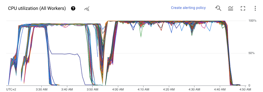
I checked if CPU utilization was on an acceptable level, and it was.

The following diagram from Dataflow UI presents CPU utilization on All Workers in terms of the CPU utilization for all cores on a single App Engine flexible instance. So it gives us an idea of how the CPU is utilized on each virtual machine.

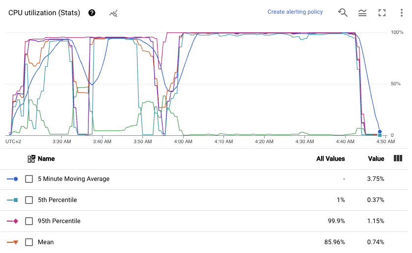
We could also take a look at the same data presented in terms of statistical metrics.

From the given graph I could see that mean utilization of the CPU was around 85%, which is a good score. The result is affected by two shuffle stages, when we need to send data around the cluster (usually network is a small bottleneck here). CPU tends to be idle while shuffling data using Dataflow Shuffle Service.

So CPU resources are not underutilized. We use almost all of what we pay for.

Memory utilization #

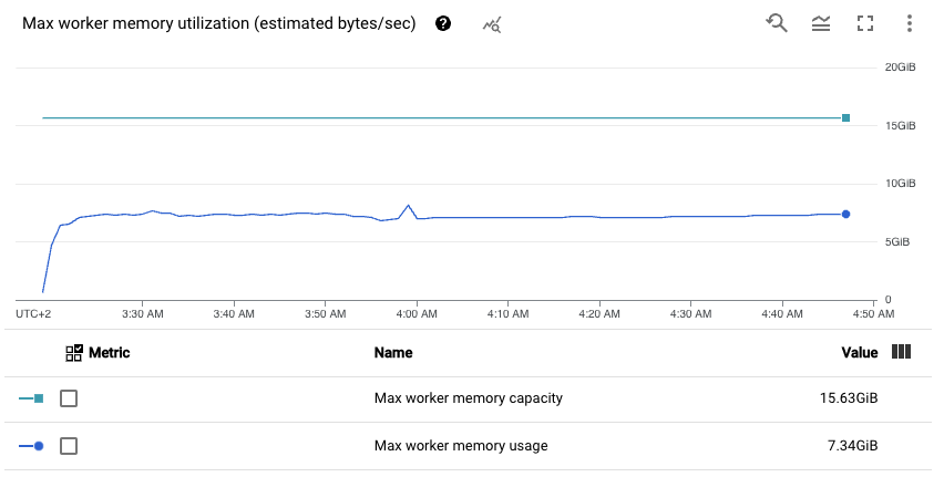
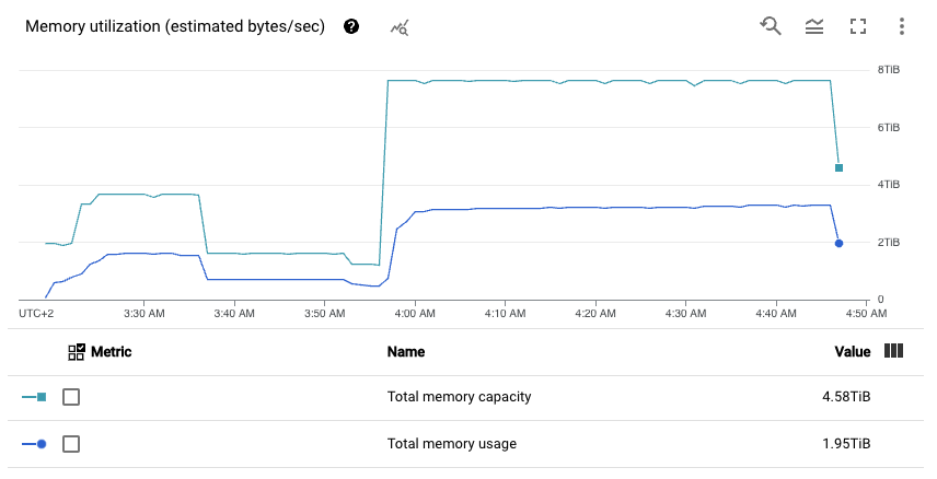
In the end I checked memory usage. I saw that we did not use all the memory which we were paying for. Let’s take a look at the following two graphs. The first one shows maximal memory utilization among all the workers.

The second one shows memory utilization statistics among all the worker nodes.

The first one presents average memory usage on a worker node, the second one presents overall memory usage among the whole cluster. We clearly see that we only use around 50% of the memory. Bingo, we pay for memory that we do not use.

Improving memory utilization #

Usually there are two ways of improving memory utilization:

Change CPU to memory ratio on worker nodes.
Decrease the amount of worker nodes.

I’ve decided to change the CPU to memory ratio rather than decrease the number of worker nodes. I did not want to compromise on scalability and time needed to perform a job.

Test on a 3% subsample of input data has given the following cost of data processing:

n2-standard-4: $9.48
n2-highcpu-8: $8.52 (~ 10% less than original price)
n2d-highcpu-8: $8.57 (~ 10% less than original price)

We saved 10% on adjusting CPU and memory ratio. It results in around $12,700 of estimated savings per year (10% of $127,000 annual cost).

Hypothesis	Savings¹
[1] Physical resources are underutilized	$12,700

Hypothesis testing: physical resources has not the best price-to-performance ratio #

I assumed that the current virtual machine type (n2-standard-4) has not the best price-to-performance ratio. To check performance of different virtual machine types I used CoreMark scores provided by Google Cloud itself.

Based on CoreMark scores and official Google Cloud VM pricing, I prepared a table which would help me choose the VM type with the best price-to-performance ratio. The most important column is “price per 1 mln points” — how much I need to pay on average to score 1 mln points. I used official VM instance prices from Google Cloud site from region europe-west1.

Virtual Machine Type	Points in ScoreMark²	Price per hour³	Price per 1 mln points
n2-standard-4	66 833 pts	$0.21	$3.20
n2-standard-8	138 657 pts	$0.43	$3.08
n2d-standard-8	164 539 pts	$0.37	$2.26
e2-standard-8	103 808 pts	$0.29	$2.84
t2d-standard-8	237 411 pts	$0.37	$1.57

As we see, another hypothesis proved to be true. We’re not using the virtual machine type with the best price-to-performance ratio - T2D. We’re using N2 machine type.

Unfortunately, at the time of writing, T2D machines do not provide CPU to memory ratios other than 3 GB per 1 vCPU. It’s still better than 4 GB per 1 vCPU, but far from 1 or 2 GB per 1 vCPU. We will check if T2D virtual machine type with 4 GB of memory per 1 CPU is cheaper than its counterparts.

Moving to a virtual machine type with better price-to-performance ratio #

I performed several tests on a small scale (3% subsample of input data) with T2D machine types. Let’s take a look at them.

n2-standard-4 + HDD: $9.48
n2-highcpu-8 + HDD: $8.52 (~ 10% less than original price)
n2d-highcpu-8 + HDD: $8.57 (~ 10% less than original price)
t2d-standard-8 + HDD: $6.65 (~ 32% less than original price)

This way we decreased the estimated processing cost from $127,000 by $40,640 per year to $86,360 (by 32%)¹. Unfortunately, we also introduced some possible underutilized resources (memory) by changing CPU to memory ratio.

Hypothesis	Savings¹
[1] Physical resources are underutilized	$12,700
[2] Moving to a more cost-effective VM type	$27,940

Total: $40,640 of estimated savings¹

Coming back to optimization of virtual machine storage type #

As I found the most suitable virtual machine type, I was able to focus on choosing between SSD and HDD disk types. As we all know, HDDs are much slower than SSDs, especially in terms of random read/write. For processes where we do not heavily use storage I/O operations there’s no need to move to more expensive SSDs.

I decided to check if we should use cheaper and slower HDDs or more expensive and faster SSDs. I run the pipeline (3% of input data size) with HDD and SSD disks. Here are the results for different VM families:

n2-standard-4 + HDD: $9.48
n2-highcpu-8 + HDD: $8.52 (~ 10% less than original price)
n2d-highcpu-8 + HDD: $8.57 (~ 10% less than original price)
t2d-standard-8 + HDD: $6.65 (~ 32% less than original price)
t2d-standard-8 + SSD: $5.64 (~ 41% less than original price)

This way we decreased the estimated processing cost from $127,000 by $52,070 per year to $74,930 (by 41%)¹.

Hypothesis	Savings¹
[1] Physical resources are underutilized	$12,700
[2] Moving to a more cost-effective VM type	$27,940
[3] Changing VM disk type to SSD	$11,430

Total: $52,070 of estimated savings¹

Hypothesis testing: configuration of the Dataflow job is not optimal #

Dataflow, in comparison to Apache Spark, leaves us with almost no configuration options to be changed. It’s good because in Dataflow you get very decent out-of-the-box settings. The single option which I wanted to tune was if we should use Shuffle Service. Shuffle Service is a serverless tool that facilitates data shuffling around the cluster, thus relieving worker nodes from this task. Also, node preemption is not so painful because Shuffle Service stores data in external storage independent of worker nodes. But it comes at a price.

Cost breakdown of processing 3% input dataset using virtual machine t2d-standard-8 with SSD disk is presented below³:

Cost of CPU: $2.47
Cost of memory: $0.70
Cost of SSD disk: $0.16
Cost of shuffle service: $2.32
Overall cost: $5.64

Thus, we see that the cost of the shuffle service plays an important role - it’s more than 40% of the overall cost. Let’s do an experiment and turn Shuffle Service off.

n2-standard-4 + HDD: $9.48 (original configuration)
t2d-standard-8 + SSD: $5.64 (~ 41% less than original configuration)
t2d-standard-8 + SSD + no Shuffle Service: $3.95 (~ 58% less than original configuration)

By turning off Shuffle Service we achieved a much lower cost. As a bonus, our memory utilization increased to almost 100%, because we use worker nodes to perform a shuffle. So we eliminated an underutilized T2D issue connected with a CPU to memory ratio. Node preemption is not a problem since we’re not utilizing preemptible VMs.

I must also add that turning off external shuffle service may not always result in lower cost. It depends on many factors, and you should test it on your own data pipeline. Also, you need to take into consideration that the job will usually require more resources (CPU, memory) once you turn off external shuffle service.

This way we decreased the estimated processing cost from $127,000 by $73,660 per year to $53,340 (by 58%)¹. So it’s now less than half of the initial cost¹.

Hypothesis	Savings¹
[1] Physical resources are underutilized	$12,700
[2] Moving to a more cost-effective VM type	$27,940
[3] Changing VM disk type to SSD	$11,430
[4] Turning off Shuffle Service	$21,590

Total: $73,660 of estimated savings¹

Note: Why did we not use Dataflow FlexRS which could lower the processing price by combining preemptible and regular VMs?

We did not test it due to how scheduling in FlexRS works. When you schedule a Dataflow FlexRS job you do not know the exact start time, the only one promise from FlexRS is that the job will start within 6 hours (documentation notes from Google Cloud website on that). Our data pipeline must start at specified time and having a 6 hour delay is not acceptable.

Final test on a full dataset #

My last task was to test findings from subsampled input dataset (3%) tests on the full dataset (without subsampling). Here are the costs of processing a full dataset for a single day:

Configuration	Processing cost for one day on a full dataset
n2-standard-4 + HDD	$350.02
t2d-standard-8 + SSD + shuffle service turned off	$134.14 (~ 62% less than original price)

As we see, the predicted gain from subsampling was achieved, and savings are even 3 pp higher than estimated. For reference: we estimated, based on runs with 3% of input size, that we will achieve a roughly 58% cost reduction.

Initial annual cost: $127,000
Estimated annual cost after optimization: $48,260
Total estimated annual savings: $78,740

Presented figures are only estimates based on a single run and extrapolated to the whole year. To know the exact savings we will need to run the processing pipeline over a year, which hasn’t been done yet.

Summary #

We achieved excellent outcome without even touching the processing code. Speculative approach provided good results. There may still be some space for optimization, but within the timeframe I was given, I treat these results as first-rate and do not find any more reasons to further optimize the environment and configuration of the Dataflow job.

Also, specified strategies do not have to lead to cost optimizations in other pipelines. As every data pipeline is different, some changes which brought cost reduction in this example may result in increased processing cost in different data pipelines. What is most important in this article: how to approach cost optimization of a data pipeline, not which type of resources to choose.

Presented figures are only estimates based on a single run (with only 3% of input data) and extrapolated to the whole year with the assumption that processing the whole dataset will result in the same relative savings as processing 3% of source data. ↩ ↩² ↩³ ↩⁴ ↩⁵ ↩⁶ ↩⁷ ↩⁸ ↩⁹ ↩¹⁰ ↩¹¹
CoreMark results from CoreMark scores provided by Google Cloud itself, retrieved on 04/05/2024. ↩
Official prices taken from Google Cloud site, VM instance pricing in region europe-west1, retrieved on 04/05/2024. ↩ ↩²

tech big data