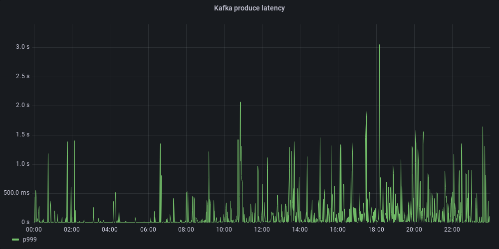
At Allegro, we use Kafka as a backbone for asynchronous communication between microservices. With up to 300k messages published and 1M messages consumed every second, it is a key part of our infrastructure. A few months ago, in our main Kafka cluster, we noticed the following discrepancy: while median response times for produce requests were in single-digit milliseconds, the tail latency was much worse. Namely, the p99 latency was up to 1 second, and the p999 latency was up to 3 seconds. This was unacceptable for a new project that we were about to start, so we decided to look into this issue. In this blog post, we would like to describe our journey — how we used Kafka protocol sniffing and eBPF to identify and remove the performance bottleneck.

The Need for Tracing

Kafka brokers expose various metrics. From them, we were able to tell that produce requests were slow for high percentiles, but we couldn’t identify the cause. System metrics were also not showing anything alarming.

To pinpoint the underlying problem, we decided to trace individual requests. By analyzing components of Kafka involved in handling produce requests, we aimed to uncover the source of the latency spikes. One way of doing that would be to fork Kafka, implement instrumentation, and deploy our custom version to the cluster. However, this would be very time-consuming and invasive. We decided to try an alternative approach.

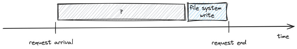
The first thing we did was finding arrival and end times for every Kafka produce request.

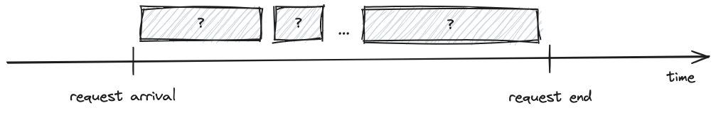Timeline of a produce request. Arrival and end times define the boundaries of the request. The components of Kafka involved in handling the request and their latencies are unknown.

Kafka uses a binary protocol over TCP to send requests from producers (and consumers) to brokers. We started by capturing the network traffic on a selected broker using tcpdump. Then we wrote a tool for analyzing the captured packets, which enabled us to list all the request and response times. In the output, we saw a confirmation of what we already knew — there were many slow produce requests taking over a second to complete. What’s more we were able to see request metadata — topic name, partition ID and message ID (our internal identifier included in Kafka headers):

ARRIVAL TIME  END TIME      LATENCY(ms)  MESSAGE_ID  TOPIC   PARTITION
12:11:36.521  12:11:37.060  538          371409548   topicA  2
12:11:36.519  12:11:37.060  540          375783615   topicB  18
12:11:36.519  12:11:37.060  540          375783615   topicB  18
12:11:36.555  12:11:37.061  505          371409578   topicC  7
12:11:36.587  12:11:37.061  473          375783728   topicD  16
12:11:36.690  12:11:37.061  370          375783907   topicB  18

With that extra knowledge in hand, we were ready to dig deeper.

Dynamic Tracing

Thanks to network traffic analysis we had arrival time, end time and metadata for each request. We then wanted to gain insights into which Kafka components were the source of latency. Since produce requests are mostly concerned with saving data, we decided to instrument writes to the underlying storage.

On Linux, Kafka uses regular files for storing data. Writes are done using ordinary write system calls — data is first stored in the page cache and then asynchronously flushed to disk. How can we trace individual file writes without modifying the source code? We can make use of dynamic tracing.

What is dynamic tracing? In Brendan Gregg’s System Performance, he uses the following analogy that we really like:

Consider an operating system kernel: analyzing kernel internals can be like venturing into a dark room, with candles […] placed where the kernel engineers thought they were needed. Dynamic instrumentation is like having a flashlight that you can point anywhere.

This basically means that it is possible to instrument arbitrary kernel code without the need to modify a user space application or the kernel itself. For example, we can use dynamic tracing to instrument file system calls to check whether they are the source of latency. To do that we can make use of a technology called BPF.

BPF (or eBPF) which stands for (extended) Berkeley Packet Filter is a technology with a rich history, but today it is a generic in-kernel execution environment [Gregg Brendan (2020). Systems Performance: Enterprise and the Cloud, 2nd Edition]. It has a wide range of applications, including networking, security and tracing tools. eBPF programs are compiled to bytecode which is then interpreted by the Linux Kernel.

There are a couple of well-established front-ends for eBPF, including BCC, bpftrace and libbpf. They can be used to write custom tracing programs, but they also ship with many useful tools already implemented. One such tool is ext4slower. It allows tracing file system operations in the ext4 file system, which is the default file system for Linux.

Tracing Kafka

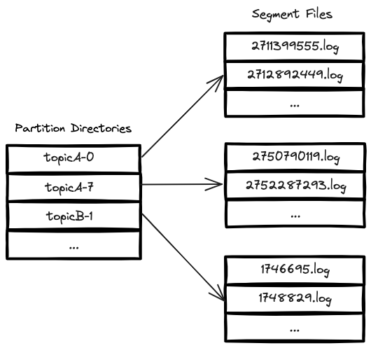
In Kafka, every partition has its own directory, named according to the pattern: topicName-partitionID. Within each of these directories, there are segment files where messages are stored. In the figure below, we can see an example of this structure. In this scenario, the broker hosts two partitions (0 and 7) for topicA and one partition (1) for topicB.

By slightly altering the ext4slower program to include parent directories, we were able to trace Kafka file system writes. For every write with a duration exceeding a specified threshold, we observed the following:

• Start time and end time
• Duration
• Thread ID (TID)
• Number of bytes written
• File offset
• Topic name
• Partition ID

Below is an example output from the program:

START TIME    END TIME      LATENCY  TID   BYTES  OFF_KB     FILE
15:37:00.627  15:37:00.785  158 ms   4478  2009   88847331   topicA-0/00000000002938697123.log
15:37:00.629  15:37:00.785  156 ms   4492  531    289315894  topicB-7/00000000001119733846.log
15:37:00.629  15:37:00.785  156 ms   4495  815    167398027  topicC-7/00000000015588371822.log
15:37:00.631  15:37:00.785  154 ms   4488  778    502626221  topicD-7/00000000004472160265.log
15:37:00.644  15:37:00.785  141 ms   4486  341    340818418  topicE-7/00000000002661443174.log
15:37:00.650  15:37:00.785  135 ms   4470  374    230883174  topicF-7/00000000006102922534.log
15:37:00.653  15:37:00.785  132 ms   4461  374    375758631  topicF-19/00000000001555977358.log

This was already very helpful since we could, based on timestamp, topic and partition, correlate produce requests from the tcpdump output with writes to the file system:

ARRIVAL TIME  END TIME      LATENCY  MESSAGE_ID  TOPIC   PARTITION
15:37:00.627  15:37:00.785  158 ms   839584818   topicA  0
15:37:00.629  15:37:00.785  156 ms   982282008   topicB  7
15:37:00.629  15:37:00.785  156 ms   398037998   topicC  7
15:37:00.631  15:37:00.785  154 ms   793357083   topicD  7
15:37:00.644  15:37:00.786  141 ms   605597592   topicE  7
15:37:00.649  15:37:00.785  136 ms   471986034   topicF  7
15:37:00.653  15:37:00.786  132 ms   190735697   topicF  19

To gain extra confidence, we wrote a tool that parses a Kafka log file, reads the records written to it (using file offset and number of bytes written), parses them, and returns their message IDs. With that, we were able to perfectly correlate incoming requests with their respective writes:

START TIME    END TIME      LATENCY  MESSAGE_ID  FILE                                TOPIC   PARTITION  BYTES  OFF_KB
15:37:00.627  15:37:00.785  158 ms   839584818   topicA-0/00000000002938697123.log   topicA  0          2009   88847331
15:37:00.629  15:37:00.785  156 ms   982282008   topicB-7/00000000001119733846.log   topicB  7          531    289315894
15:37:00.629  15:37:00.785  156 ms   398037998   topicC-7/00000000015588371822.log   topicC  7          815    167398027
15:37:00.631  15:37:00.785  154 ms   793357083   topicD-7/00000000004472160265.log   topicD  7          778    502626221
15:37:00.644  15:37:00.786  141 ms   605597592   topicE-7/00000000002661443174.log   topicE  7          341    340818418
15:37:00.649  15:37:00.785  136 ms   471986034   topicF-7/00000000006102922534.log   topicF  7          374    230883174
15:37:00.653  15:37:00.786  132 ms   190735697   topicF-19/00000000001555977358.log  topicF  19         374    375758631

From the analysis, we were able to tell that there were many slow produce requests that spent all of their time waiting for the file system write to complete.

There were however requests that didn’t have corresponding slow writes.

Kafka Lock Contention

Slow produce requests without corresponding slow writes were always occurring around the time of some other slow write. We started wondering whether those requests were perhaps queuing and waiting for something to finish. By analyzing Kafka source code, we identified a couple of places that use synchronized blocks, including those guarding log file writes.

We set out to measure how much time Kafka’s threads, processing produce requests, spend on the aforementioned locks. Our goal was to correlate periods when they were waiting on locks with writes to the file system. We considered two approaches to do that.

The first one was to use tracing again, and perhaps combine its results with the tool we already had for tracing the ext4 file system. Looking at the JDK source code we were not able to identify a connection between synchronized blocks and traceable kernel routines. Instead, we learned that JVM ships with predefined DTrace tracepoints (DTrace can be thought of as a predecessor of eBPF). These tracepoints include hotspot:monitor__contended__enter and hotspot:monitor__contended__entered, which monitor when a thread begins waiting on a contended lock and when it finally enters it. By running Kafka with the -XX:+DTraceMonitorProbes VM option and attaching to these tracepoints we were able to see monitor wait times for a given thread.

Another approach we came up with was to capture states of Kafka’s threads by running async-profiler alongside the ext4 tracing script. We would then analyze results from both tools and correlate their outputs.

After experimenting with both ideas, we ultimately chose to stick with async-profiler. It provided a clean visualization of thread states and offered more insights into JVM-specific properties of threads.

Now, let’s delve into how we analyzed a situation when a latency spike occurred, based on an example async-profiler recording, eBPF traces, and parsed tcpdump output. For brevity, we’ll focus on one Kafka topic.

By capturing network traffic on a broker, we were able to see that there were four slow produce requests to the selected topic:

ARRIVAL TIME  END TIME      LATENCY  MESSAGE_ID  TOPIC   PARTITION
17:58:00.644  17:58:00.770  126 ms   75567596    topicF  6
17:58:00.651  17:58:00.770  119 ms   33561917    topicF  6
17:58:00.655  17:58:00.775  119 ms   20422312    topicF  6
17:58:00.661  17:58:00.776  114 ms   18658935    topicF  6

However, there was only one slow file system write for that topic:

START TIME    END TIME      LATENCY  TID   BYTES  OFF_KB     FILE
17:58:00.643  17:58:00.769  126 ms   4462  498    167428091  topicF-6/00000000000966764382.log

All other writes to that topic were fast at that time:

START TIME    END TIME      LATENCY  TID   BYTES  OFF_KB     FILE
17:58:00.770  17:58:00.770  0 ms     4484  798    167451825  topicF-6/00000000000966764382.log
17:58:00.775  17:58:00.775  0 ms     4499  14410  167437415  topicF-6/00000000000966764382.log
17:58:00.776  17:58:00.776  0 ms     4467  1138   167436277  topicF-6/00000000000966764382.log

We knew that one of the fast writes was performed from a thread with ID 4484. From a thread dump, we extracted thread names and Native IDs (NIDs). Knowing that NIDs translate directly to Linux TIDs (thread IDs), we found a thread with NID 0x1184 (decimal: 4484). We determined that the name of this thread was data-plane-kafka-request-handler-24.

We searched for this thread’s activity in the async-profiler output:

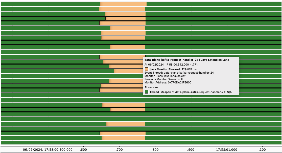Async profiler output visualized in Java Mission Control. Thread with TID 4484 is blocked on a monitor.

In the output, we saw what we suspected — a thread was waiting on a lock for approximately the same duration as the slow write occurring on another thread. This confirmed our initial hypothesis.

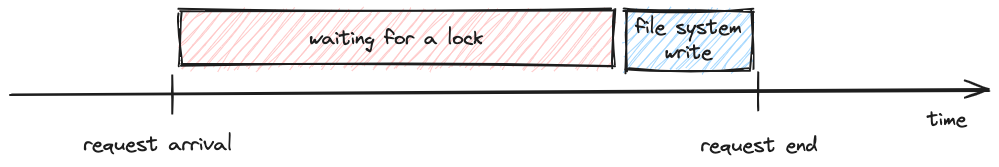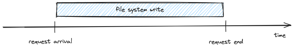
For a slow request with fast file system writes, waiting to acquire a lock turned out to be the source of latency.

Applying this technique, we analyzed numerous cases, and the results were consistent: for a slow produce request there was either a matching slow write or a thread was waiting to acquire a lock guarding access to a log file. We confirmed that file system writes were the root cause of slow produce requests.

Tracing the File System

Our original eBPF script traced only calls to the ext4_file_write_iter function. While this was sufficient to roughly determine that slow writes to the file system were causing the latency spikes, it was not enough to pinpoint which parameters of the file system needed tuning. To address this, we captured both on-CPU and off-CPU profiles of ext4_file_write_iter, using profile and offcputime, respectively. Our goal was to identify the activated paths in the kernel and then measure the latency of functions associated with them.

on-CPU profile of ext4_file_write_iter

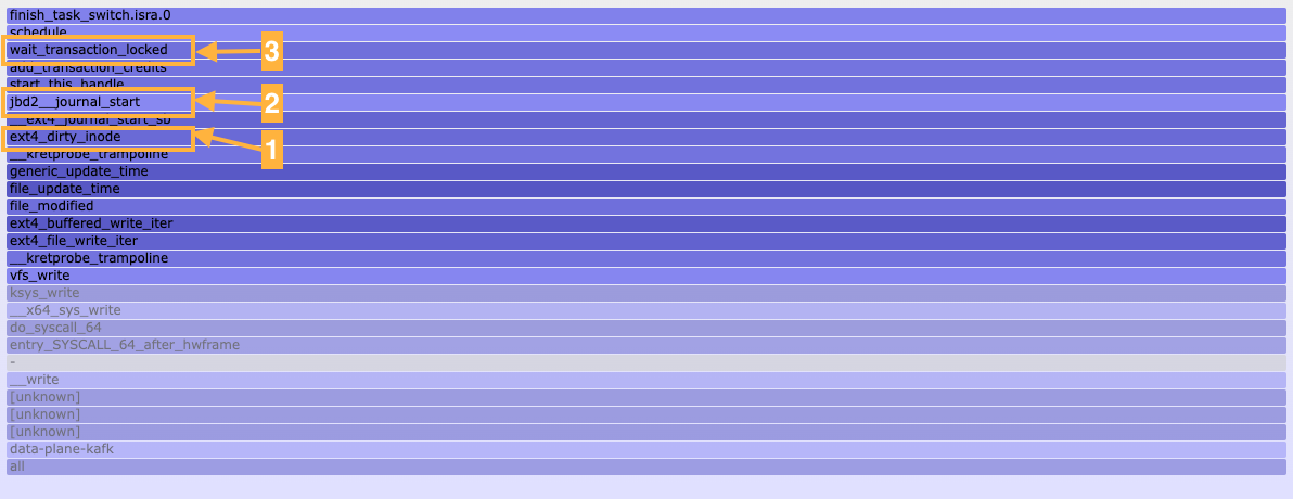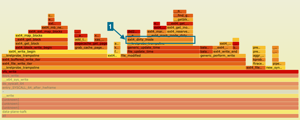
off-CPU profile of ext4_file_write_iter

We noticed that the function ext4_dirty_inode [1] was present in both flamegraphs. In the Linux kernel, the ext4_dirty_inode function is responsible for marking an inode (file or directory data structure) as being in a dirty state. A dirty inode indicates that the corresponding file’s data or metadata has been modified and needs to be synchronized with the underlying storage device, typically a disk, to ensure data consistency.

What caught our attention in the off-CPU profile was the jbd2__journal_start [2] function which is part of a journaling mechanism employed in ext4 that ensures data integrity and reliability. Journaling in ext4 involves maintaining a detailed log that records the changes before they are committed to the file system. This log, often referred to as the journal, serves as a safety net in the event of an unexpected system crash or power failure. When a file system operation occurs, such as creating, modifying, or deleting a file, ext4 first records this change in the journal. Subsequently, the actual file system structures are updated. The process of updating the file system is known as committing the journal. During a commit, the changes recorded in the journal are applied to the file system structures in a controlled and atomic manner. In the event of an interruption, the file system can recover quickly by replaying the journal, ensuring that it reflects the consistent state of the file system.

As seen in the figure with the off-CPU profile, wait_transaction_locked [3] is the function executed before voluntarily yielding the processor, allowing the scheduler to select and switch to a different process or thread ready to run (schedule()). Guided by the comment above the wait_transaction_locked function:

Wait until running transaction passes to T_FLUSH state and new transaction can thus be started. Also starts the commit if needed. The function expects running transaction to exist and releases j_state_lock.

We searched the kernel code to identify what sets the T_FLUSH flag. The only place that we discovered was within the jbd2_journal_commit_transaction function executed periodically by a kernel journal thread. Consequently, we decided to trace this function to explore any correlation between its latency and the latency of ext4_dirty_inode. The obtained results aligned precisely with our expectations – namely, a high latency in jbd2_journal_commit_transaction translates to a high latency in ext4_dirty_inode. The details of our findings are presented below:

START TIME    END TIME      LATENCY  FUNCTION
19:35:24.503  19:35:24.680  176 ms   jbd2_journal_commit_transaction
19:35:24.507  19:35:24.648  141 ms   ext4_dirty_inode
19:35:24.508  19:35:24.648  139 ms   ext4_dirty_inode
19:35:24.514  19:35:24.648  134 ms   ext4_dirty_inode
...
19:38:14.508  19:38:14.929  420 ms   jbd2_journal_commit_transaction
19:38:14.511  19:38:14.868  357 ms   ext4_dirty_inode
19:38:14.511  19:38:14.868  357 ms   ext4_dirty_inode
19:38:14.512  19:38:14.868  356 ms   ext4_dirty_inode
...
19:48:39.475  19:48:40.808  1332 ms  jbd2_journal_commit_transaction
19:48:39.477  19:48:40.757  1280 ms  ext4_dirty_inode
19:48:39.487  19:48:40.757  1270 ms  ext4_dirty_inode
19:48:39.543  19:48:40.757  1213 ms  ext4_dirty_inode
...

ext4 Improvements Monitoring

Having identified journal commits as the cause of slow writes, we started thinking how to alleviate the problem. We had a few ideas, but we were wondering how we would be able to observe improvements. Up until that point, we relied on command-line tools and analyzing their output for short time ranges. We wanted to be able to observe the impact of our optimizations over longer periods.

To report traced functions latency over long periods, we used ebpf_exporter, a tool that exposes eBPF-based metrics in Prometheus format. We were then able to visualize traces in Grafana. For example, maximum ext4 write latency for a given broker:

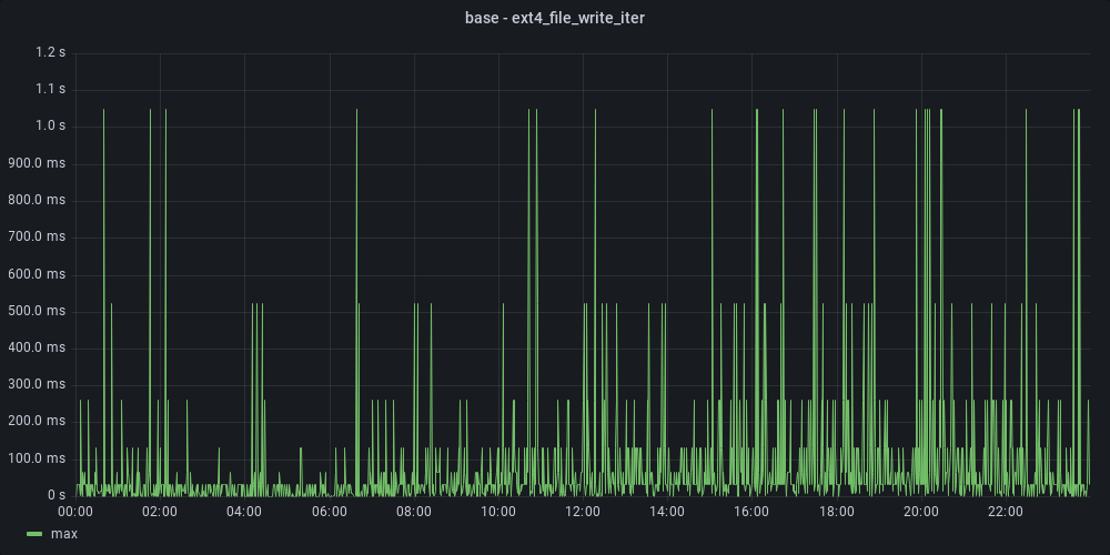
With that, we were able to run brokers with different configurations and observe their write latency over time.

ext4 Improvements

Let’s go back to ext4. We knew that journal commits were the source of latency. By studying ext4 documentation, we identified a few possible solutions for improving the performance:

1. Disabling journaling
2. Decreasing the commit interval
3. Changing the journaling mode from data=ordered to data=writeback
4. Enabling fast commits

Let’s discuss each of them.

Disabling Journaling

If journaling is the source of high latency, why not disable it completely? Well, it turns out that journaling is there for a reason. Without journaling, we would risk long recovery in case of a crash. Thus, we quickly ruled out this solution.

Decreasing the Commit Interval

ext4 has the commit mount parameter which tells how often to perform commits. It has the default value of 5 seconds. According to the ext4 documentation:

This default value (or any low value) will hurt performance, but it’s good for data-safety. […] Setting it to very large values will improve performance.

However, instead of increasing the value we decided to decrease it. Why? Our intuition was that by performing commits more frequently we would make them “lighter” which would make them faster. We would trade throughput for lower latency. We experimented with commit=1, and commit=3 but observed no significant differences.

Changing the Journaling Mode from data=ordered to data=writeback

ext4 offers three journaling modes: journal, ordered and writeback. The default mode is ordered and compared to the most performant mode, writeback, it guarantees that the data is written to the main file system prior to the metadata being committed to the journal. As mentioned in docs, Kafka does not rely on this property, so switching the mode to writeback should reduce latency.

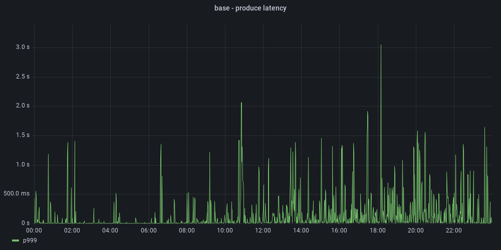
We switched the journaling mode on one of the brokers, and indeed, we observed latency improvements:

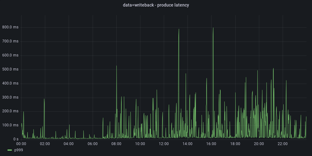With data=writeback, p999 decreased from 3 seconds to 800 milliseconds.

Enabling Fast Commit

When reading about ext4 journaling, we stumbled upon an article describing a new feature introduced in Linux 5.10 called fast commits. As explained in the article, fast commit is a lighter-weight journaling method that could result in performance boost for certain workloads.

We enabled fast commit on one of the brokers. We noticed that max write latency decreased significantly. Diving deeper we found out that on a broker with fast commit enabled:

• The latency of jdb2_journal_commit_transaction decreased by an order of magnitude. This meant that periodic journal commits were indeed much faster thanks to enabling fast commits.
• Slow ext4 writes occurred at the same time when there was a spike in latency of jbd2_fc_begin_commit. This method is part of the fast commit flow. It became the new source of latency but its maximum latency was lower than that of jdb2_journal_commit_transaction without fast commits.

Comparison of maximum latency [s] of ext4 writes for brokers without and with fast commit.

Lower file system write latency, in turn, resulted in reduced produce latency:

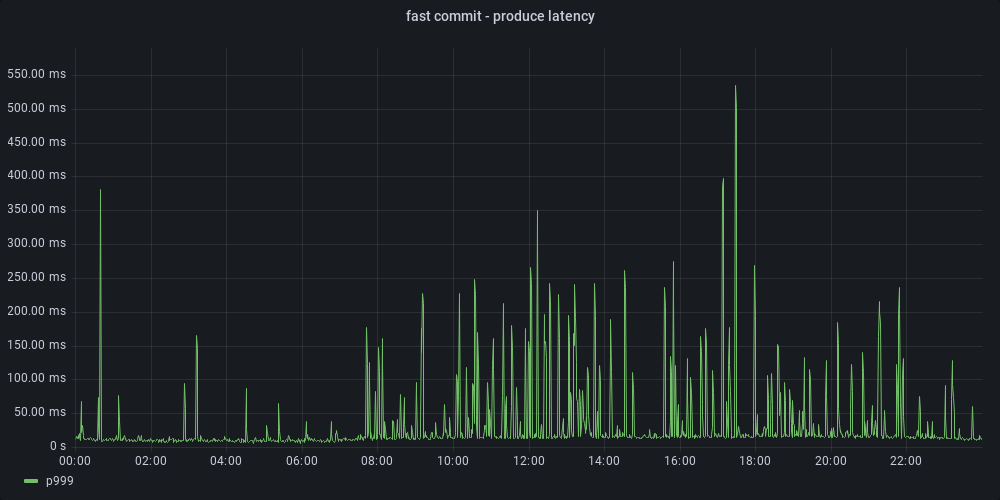With fast commit enabled, produce P999 latency went down from 3 seconds to 500 milliseconds

Summary

To summarize, we’ve tested the following ext4 optimizations:

• Decreasing the commit interval
• Changing the journaling mode to data=writeback
• Enabling fast commit

We observed that both data=writeback and fast commit significantly reduced latency, with fast commit having slightly lower latency. The results were promising, but we had higher hopes. Thankfully, we had one more idea left.

XFS

While researching the topic of journaling in ext4, we stumbled upon a few sources suggesting that the XFS file system, with its more advanced journaling, is well-suited for handling large files and high-throughput workloads, often outperforming ext4 in such scenarios. Kafka documentation also mentions that XFS has a lot of tuning already in place and should be a better fit than the default ext4.

We migrated one of the brokers to the XFS file system. The results were impressive. The thing that was very distinctive compared to the aforementioned ext4 optimizations was the consistency of XFS performance. While other broker configurations experienced p999 latency spikes throughout the day, XFS – with its default configuration – had only a few hiccups.

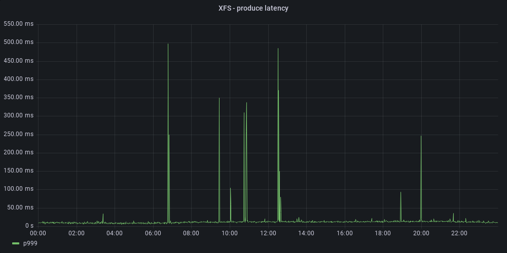
After a couple of weeks of testing, we were confident that XFS was the best choice. Consequently, we migrated all our brokers from ext4 to XFS.

Summary

Using a combination of packet sniffing, eBPF, and async-profiler we managed to identify the root cause of slow produce requests in our Kafka cluster. We then tested a couple of solutions to the problem: data=writeback journaling mode, fast commits, and changing the file system to XFS. The results of these optimizations are visualized in the heatmap below:

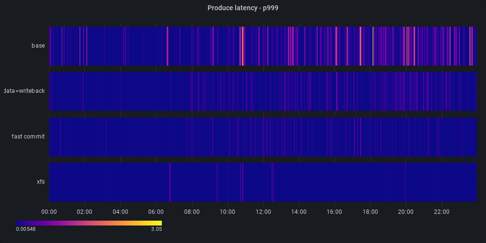
Ultimately, we found XFS to be the most performant and rolled it out to all of our brokers. With XFS, the number of produce requests exceeding 65ms (our SLO) was lowered by 82%.

Here are some of the lessons we learned along the way:

• eBPF was extremely useful during the analysis. It was straightforward to utilize one of the pre-existing tools from bcc or bpftrace. We were also able to easily modify them for our custom use cases.
• ebpf_exporter is a great tool for observing trace results over longer periods of time. It allows to expose Prometheus metrics based on libbpf programs.
• p99 and p999 analysis is sometimes not enough. In our case, the p999 latency of file system writes was less than 1ms. It turned out that a single slow write could cause lock contention and a cascade of slow requests. Without tracing individual requests, the root cause would have been very hard to catch.

We hope that you found this blog post useful, and we wish you good luck in your future performance analysis endeavors!

Acknowledgments

We would like to thank our colleague Dominik Kowalski for performing the XFS migration and applying the ext4 configuration changes to the Kafka cluster.