B-tree is a structure that helps to search through great amounts of data. It was invented over 40 years ago, yet it is still employed by the majority of modern databases. Although there are newer index structures, like LSM trees, B-tree is unbeaten when handling most of the database queries.

After reading this post, you will know how B-tree organises the data and how it performs search queries.

Origins

In order to understand B-tree let’s focus on Binary Search Tree (BST) first.

Wait, isn’t it the same?

What does “B” stand for then?

According to wikipedia.org, Edward M. McCreight, the inventor of B-tree, once said:

“the more you think about what the B in B-trees means, the better you understand B-trees.”

Confusing B-tree with BST is a really common misconception. Anyway, in my opinion, BST is a great starting point for reinventing B-tree. Let’s start with a simple example of BST:

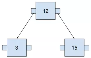
The greater number is always on the right, the lower on the left. It may become clearer when we add more numbers.

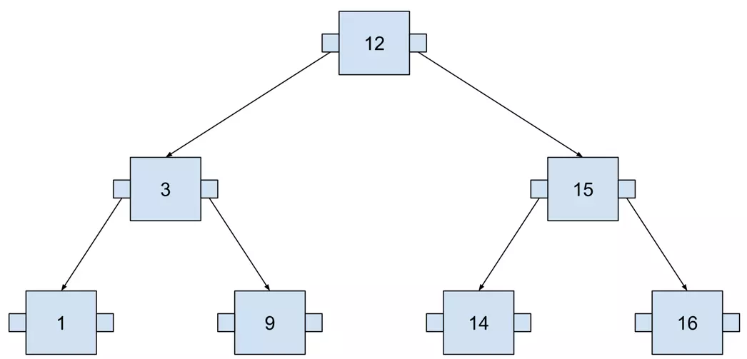
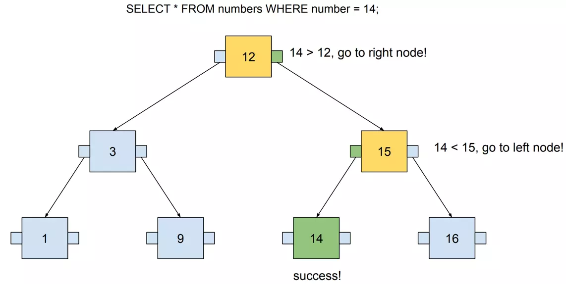
This tree contains seven numbers, but we need to visit at most three nodes to locate any number. The following example visualizes searching for 14. I used SQL to define the query in order to think about this tree as if it were an actual database index.

Hardware

In theory, using Binary Search Tree for running our queries looks fine. Its time complexity (when searching) is \(O(log n)\), same as B-tree. However, in practice, this data structure needs to work on actual hardware. An index must be stored somewhere on your machine.

The computer has three places where the data can be stored:

• CPU caches
• RAM (memory)
• Disk (storage)

The cache is managed fully by CPUs. Moreover, it is relatively small, usually a few megabytes. Index may contain gigabytes of data, so it won’t fit there.

Databases vastly use Memory (RAM). It has some great advantages:

• assures fast random access (more on that in the next paragraph)
• its size may be pretty big (e.g. AWS RDS cloud service provides instances with a few terabytes of memory available).

Cons? You lose the data when the power supply goes off. Moreover, when compared to the disk, it is pretty expensive.

Finally, the cons of a memory are the pros of a disk storage. It’s cheap, and data will remain there even if we lose the power. However, there are no free lunches! The catch is that we need to be careful about random and sequential access. Reading from the disk is fast, but only under certain conditions! I’ll try to explain them simply.

Random and sequential access

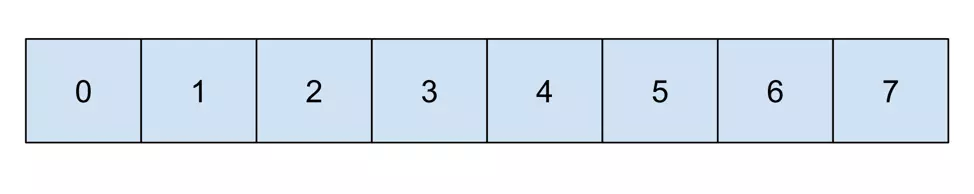
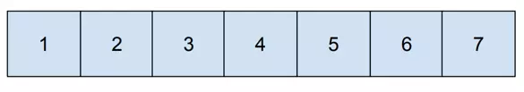
Memory may be visualized as a line of containers for values, where every container is numbered.

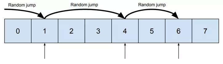
Now let’s assume we want to read data from containers 1, 4, and 6. It requires random access:

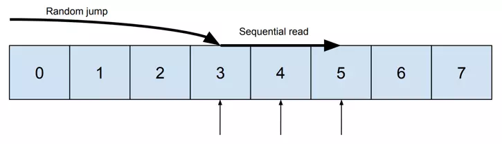
And then let’s compare it with reading containers 3, 4, and 5. It may be done sequentially:

The difference between a “random jump” and a “sequential read” can be explained based on Hard Disk Drive. It consists of the head and the disk.

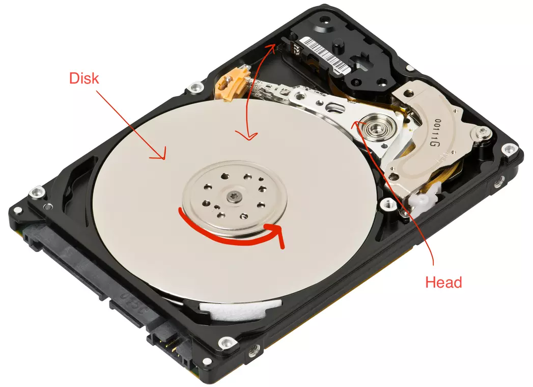
“Random jump” requires moving the head to the given place on the disk. “Sequential read” is simply spinning the disk, allowing the head to read consecutive values. When reading megabytes of data, the difference between these two types of access is enormous. Using “sequential reads” lowers the time needed to fetch the data significantly.

Differences in speed between random and sequential access were researched in the article “The Pathologies of Big Data” by Adam Jacobs, published in Acm Queue. It revealed a few mind-blowing facts:

• Sequential access on HDD may be hundreds of thousands of times faster than random access. 🤯
• It may be faster to read sequentially from the disk than randomly from the memory.

Who even uses HDD nowadays? What about SSD? This research shows that reading fully sequentially from HDD may be faster than SSD. However, please note that the article is from 2009 and SSD developed significantly through the last decade, thus these results are probably outdated.

To sum up, the key takeaway is to prefer sequential access wherever we can. In the next paragraph, I will explain how to apply it to our index structure.

Optimizing a tree for sequential access

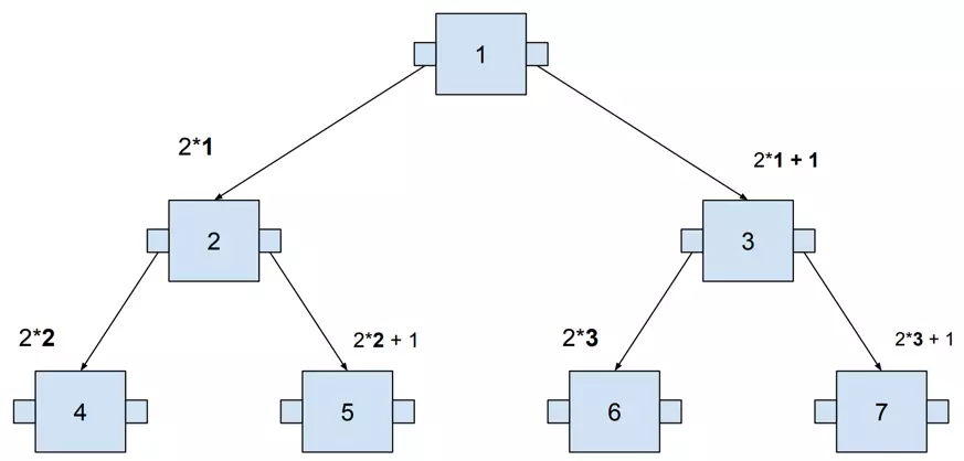
Binary Search Tree may be represented in memory in the same way as the heap:

• parent node position is \(i\)
• left node position is \(2i\)
• right node position is \(2i+1\)

That’s how these positions are calculated based on the example (the parent node starts at 1):

According to the calculated positions, nodes are aligned into the memory:

Do you remember the query visualized a few chapters ago?

That’s what it looks like on the memory level:

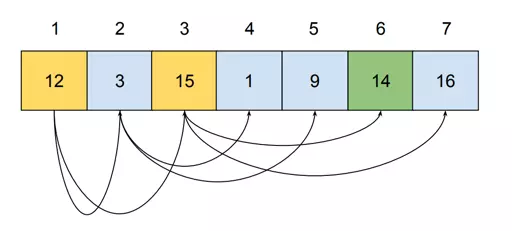
When performing the query, memory addresses 1, 3, and 6 need to be visited. Visiting three nodes is not a problem; however, as we store more data, the tree gets higher. Storing more than one million values requires a tree of height at least 20. It means that 20 values from different places in memory must be read. It causes completely random access!

Pages

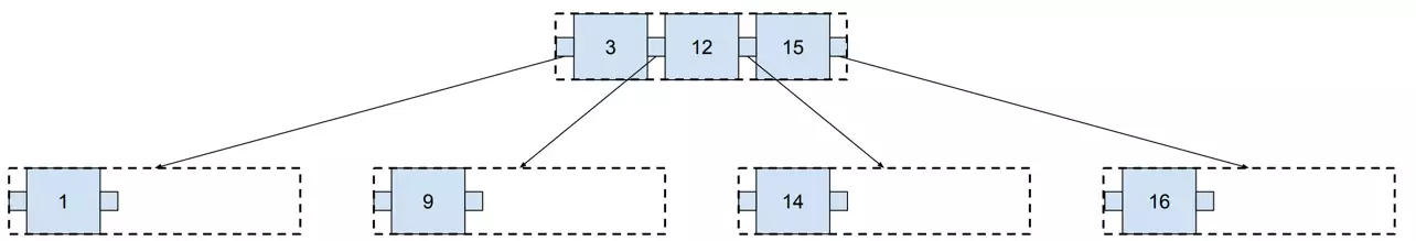
While a tree grows in height, random access is causing more and more delay. The solution to reduce this problem is simple: grow the tree in width rather than in height. It may be achieved by packing more than one value into a single node.

It brings us the following benefits:

• the tree is shallower (two levels instead of three)
• it still has a lot of space for new values without the need for growing further

The query performed on such index looks as follows:

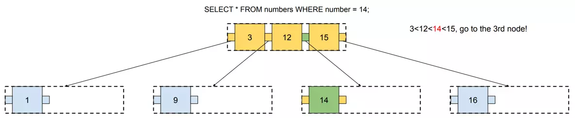
Please note that every time we visit a node, we need to load all its values. In this example, we need to load 4 values (or 6 if the tree is full) in order to reach the one we are looking for. Below, you will find a visualization of this tree in a memory:

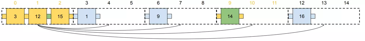
Compared to the previous example (where the tree grows in height), this search should be faster. We need random access only twice (jump to cells 0 and 9) and then sequentially read the rest of values.

This solution works better and better as our database grows. If you want to store one million values, then you need:

• Binary Search Tree which has 20 levels

OR

• 3-value node Tree which has 10 levels

Values from a single node make a page. In the example above, each page consists of three values. A page is a set of values placed on a disk next to each other, so the database may reach the whole page at once with one sequential read.

And how does it refer to the reality? Postgres page size is 8kB. Let’s assume that 20% is for metadata, so it’s 6kB left. Half of the page is needed to store pointers to node’s children, so it gives us 3kB for values. BIGINT size is 8 bytes, thus we may store ~375 values in a single page.

Assuming that some pretty big tables in a database have one billion rows, how many levels in the Postgres tree do we need to store them? According to the calculations above, if we create a tree that can handle 375 values in a single node, it may store 1 billion values with a tree that has only four levels. Binary Search Tree would require 30 levels for such amount of data.

To sum up, placing multiple values in a single node of the tree helped us to reduce its height, thus using the benefits of sequential access. Moreover, a B-tree may grow not only in height, but also in width (by using larger pages).

Balancing

There are two types of operations in databases: writing and reading. In the previous section, we addressed the problems with reading the data from the B-tree. Nonetheless, writing is also a crucial part. When writing the data to a database, B-tree needs to be constantly updated with new values.

The tree shape depends on the order of values added to the tree. It’s easily visible in a binary tree. We may obtain trees with different depths if the values are added in an incorrect order.

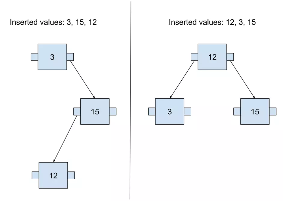
When the tree has different depths on different nodes, it is called an unbalanced tree. There are basically two ways of returning such a tree to a balanced state:

1. Rebuilding it from the very beginning just by adding the values in the correct order.
2. Keeping it balanced all the time, as the new values are added.

B-tree implements the second option. A feature that makes the tree balanced all the time is called self-balancing.

Self-balancing algorithm by example

Building a B-tree can be started simply by creating a single node and adding new values until there is no free space in it.

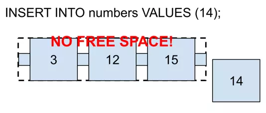
If there is no space on the corresponding page, it needs to be split. To perform a split, a „split point” is chosen. In that case, it will be 12, because it is in the middle. The „Split point” is a value that will be moved to the upper page.

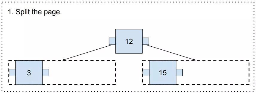
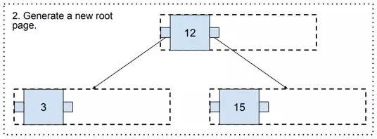
Now, it gets us to an interesting point where there is no upper page. In such a case, a new one needs to be generated (and it becomes the new root page!).

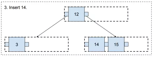
And finally, there is some free space in the three, so value 14 may be added.

Following this algorithm, we may constantly add new values to the B-tree, and it will remain balanced all the time!

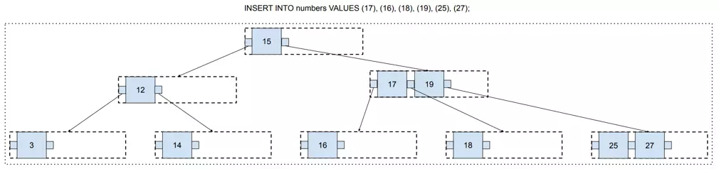
At this point, you may have a valid concern that there is a lot of free space that has no chance to be filled. For example, values 14, 15, and 16, are on different pages, so these pages will remain with only one value and two free spaces forever.

It was caused by the split location choice. We always split the page in the middle. But every time we do a split, we may choose any split location we want.

Postgres has an algorithm that is run every time a split is performed! Its implementation may be found in the _bt_findsplitloc() function in Postgres source code. Its goal is to leave as little free space as possible.

Summary

In this article, you learned how a B-tree works. All in all, it may be simply described as a Binary Search Tree with two changes:

• every node may contain more than one value
• inserting a new value is followed by a self-balancing algorithm.

Although the structures used by modern databases are usually some variants of a B-tree (like B+tree), they are still based on the original conception. In my opinion, one great strength of a B-tree is the fact that it was designed directly to handle large amounts of data on actual hardware. It may be the reason why the B-tree has remained with us for such a long time.