• Label noise is ever-present in machine learning practice.
• Allegro datasets are no exception.
• We compared 7 methods for training classifiers robust to label noise.
• All of them improved the model’s performance on noisy datasets.
• Some of the methods decreased the model’s performance in the absence of label noise.

What is label noise and why does it matter?

In the scope of supervised machine learning, specifically in classification tasks, the problem of label noise is of critical importance. It involves cases of incorrectly labelled training data. For example, let’s say that we want to train a classification model to distinguish cats from dogs. For that purpose, we compose a training dataset with images labelled as either cat or dog. The labelling process is usually performed by human annotators, who almost certainly produce some labelling errors. Unfortunately, human annotators can be confused by poor image quality, ambiguous image contents, or simply click the wrong item. As such, we inevitably end up with a dataset where some percentage of cats are labelled as dogs and vice versa (Figure 1).

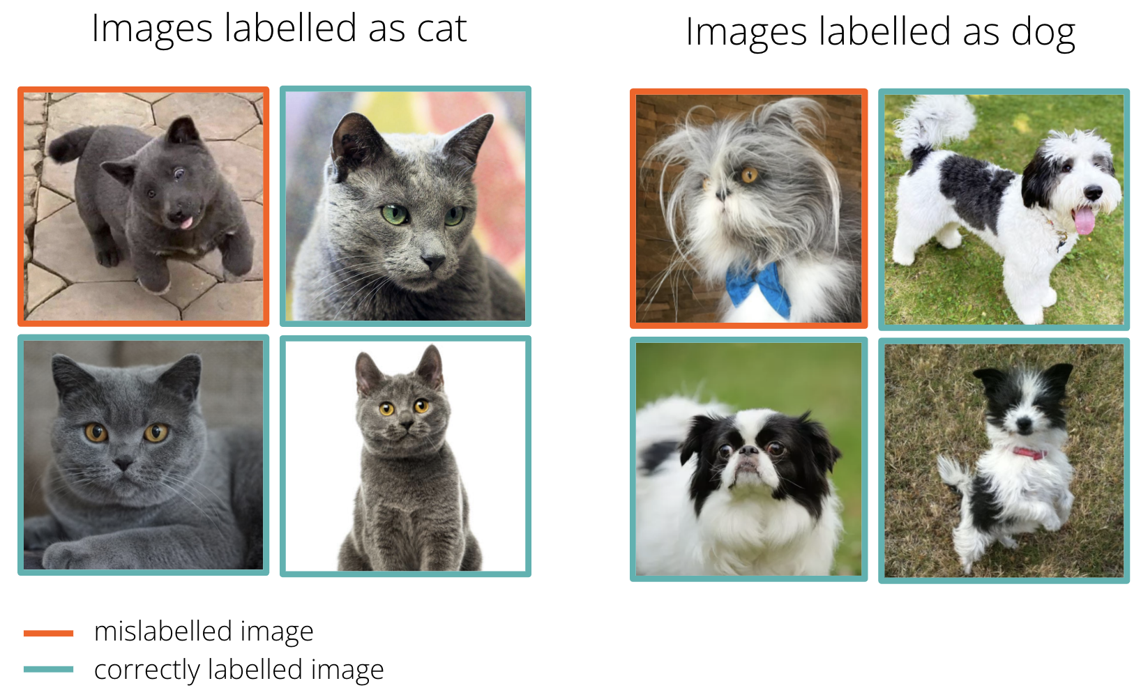
Figure 1. An example of label noise in a binary classification dataset. Some images in both categories were mislabelled by human annotators, which introduces noise to the training dataset.

Consequently, the model trained with such data learns partially wrong associations, which then can lead to incorrect predictions for new images. The more label noise we have, the more we confuse the model during training. We can measure this by evaluating the classification error on a held-out test dataset (Figure 2). It is clear that for high noise levels, it is very hard to recover the true training signal from the corrupted training data.

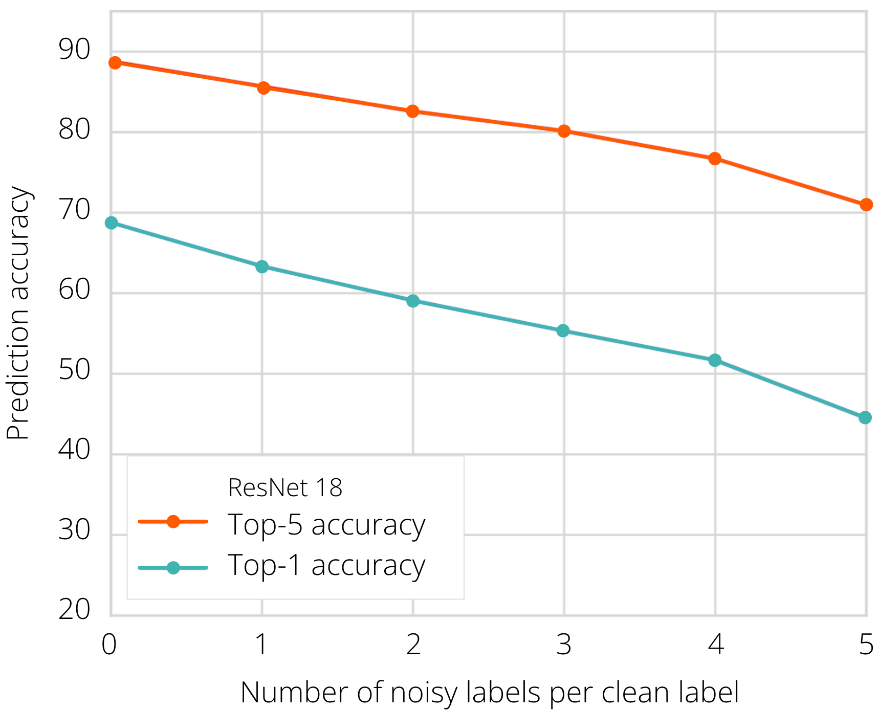
Figure 2. Test accuracy as a function of label noise percentage. The X axis indicates the ratio of mislabelled to correctly labelled examples. The dataset used here was ImageNet, corrupted with synthetic label noise. Image source: ¹.

How can this problem be mitigated? One approach is to simply put more effort into the labelling process — we can let multiple annotators label each data point and then evaluate the cross-annotator agreement. With enough time and effort, we hope to obtain a dataset free of label noise. However, in practice this approach is rarely feasible due to large volumes of training data and the need for efficient turnaround of machine learning projects. Consequently, we need a different approach for handling corrupted training data, i.e. ML models robust to label noise.

In the context of this blog post, we define robustness as the model’s ability to efficiently learn in the presence of corrupted training data. In other words, a robust model can recover the correct training signal and ignore the noise, so that it does not overfit to the corrupted traning set and can generalise during prediction. A major challenge in this regard is the difficulty to estimate the proportion of label noise in real-world data. As such, robust models are expected to handle varying amounts of label noise.

How to train a robust classifier?

We can improve the robustness of deep neural networks (DNNs) with a few tips and tricks presented in the recent literature on Learning from Noisy Data. In general, there are three approaches to boosting the model’s resistance to noisy labels (Figure 3):

• Robust loss function boosting the training dynamics in the presence of noise.
• Implicit regularisation of the network aiming at decreasing the impact of noisy labels.
• Filtration of noisy data samples during the training or at the pre-training stage.

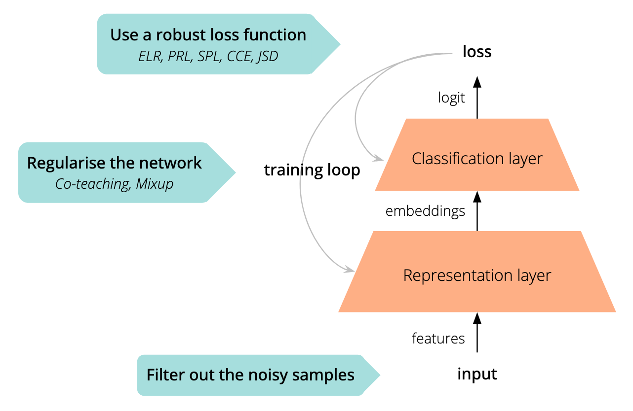
Figure 3. Strategies for robustness. In this blog post, we focused on two main approaches improving model robustness: utilisation of a robust loss function and implicit regularisation.

In the scope of this blog post, we present seven different methods that are strong baselines for improving the generalisation of classifiers in the presence of label noise.

Robust loss function

Self-Paced Learning (SPL)

The authors of Self-Paced Learning² noticed that large per-sample loss might be an indication of label corruption, especially in the latter stages of training. Clean labels should be easy to learn, while corrupted labels would appear as difficult, resulting in a high per-sample loss.

SPL proposes to exclude some predefined ratio of examples from the batch depending on their per-sample loss values (Figure 4a). Usually, the ratio is set as the estimated noise level in the dataset.

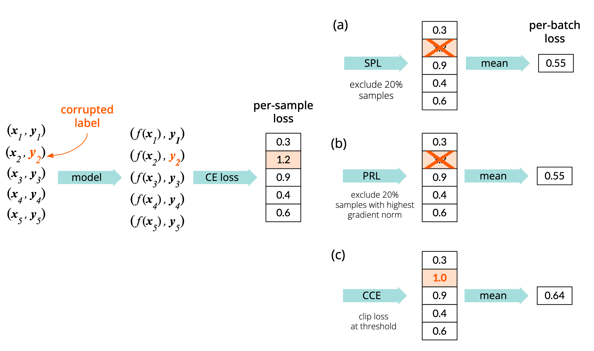
Figure 4. Comparison of loss filtration methods (SPL, PRL and CCE, see below). While SPL and PRL exclude samples from loss calculation, CCE decreases the impact of potentially corrupted labels by clipping the per-sample loss values. Orange colour indicates candidate noisy samples.

Provably Robust Learning (PRL)

Provably Robust Learning³ derives from the ideas presented in the SPL paper, but the authors state that corrupted labels should be detected depending on the gradient norm, instead of per-sample loss (Figure 4b). The underlying intuition is that corrupted samples provoke the optimiser to make inadequately large steps in the optimisation space. The rest of the logic is the same as in SPL.

Clipped Cross-Entropy (CCE)

Rejection of samples might not be optimal from the training’s point of view, because DNNs need vast amounts of data to be able to generalise properly. Therefore, Clipped Cross-Entropy doesn’t exclude the most contributing samples from the batch, but rather alleviates their impact by clipping the per-sample loss to a predefined value (Figure 4c).

Early Learning Regularisation (ELR)

It has been recently observed that DNNs first fit clean samples, and then start memorising the noisy ones. This phenomenon reduces the generalisation properties of the model, distracting it from learning true patterns present in the data. Early Learning Regularisation⁴ mitigates memorisation with two tricks:

• Temporal ensembling of targets: during the training step \([k]\), the original targets \(\pmb{\text{t}}\) are mixed with the model’s predictions \(\pmb{\text{p}}\) from previous training steps. This prevents the gradient from diverging hugely between subsequent steps. This trick is well-known in semi-supervised learning⁵:

\[\pmb{\text{t}}^{[k]} = \left(\beta\ \pmb{\text{t}}^{[k-1]} + (1-\beta)\ \pmb{\text{p}}^{[k-1]}\right)\]

• Explicit regularisation: an extra term is added to the default cross-entropy loss \(\mathcal{L}_{CE}(\Theta)\) that allows refinement of the early-learnt concepts, but penalises drastically contradicting predictions.

\[\mathcal{L}_{ELR}(\Theta)=\mathcal{L}_{CE}(\Theta) + \frac{\lambda}{n} \sum\text{log}(1-\langle \pmb{\text{p}}, \pmb{\text{t}} \rangle)\]

Thus, the gradient gets a boost for the clean samples, while the impact of noisy samples is neutralised by temporal ensembling.

Jensen-Shannon Divergence Loss (JSD)

The authors of Jensen-Shannon Divergence Loss ⁶ take yet another approach to loss construction, which is inspired by an empirical comparison between Cross-Entropy (CE) and Mean Absolute Error (MAE) loss. CE is known for its fast convergence and brilliant training dynamics, while MAE provides spectacular robustness at the price of slow convergence.

Englesson et al. came up with the idea to use Jensen-Shannon Divergence, which is a proven generalisation of CE and MAE loss (Figure 5). JSD uses Kullback-Leibler Divergence \(\text{D}_{\text{KL}}\) between the target labels \(\pmb{y}\) and predictions of the model \(f(\pmb{x})\) vs. their averaged distribution \(\pmb{m}\). Summing up, one can think of JSD as a CE with a robustness boost, or MAE with improved convergence.

\[\mathcal{L}_{\text{JS}}(\pmb{x}, \pmb{y}) = \frac{1}{Z} \left( \pi_1 \text{D}_{\text{KL}}(\pmb{y}||\pmb{m}) + (1-\pi_1) \text{D}_{\text{KL}}(f(\pmb{x})||\pmb{m}) \right)\]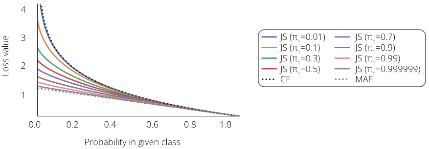

Figure 5. JSD as a generalisation of CE and MAE loss. Depending on the parameter \(\pi_1\), JSD resembles CE or MAE. Image source: ⁶.

Implicit regularisation

Co-teaching (CT)

In co-teaching ⁷, we simultaneously train two independent DNNs (Figure 6), and let them exchange examples during the training. The training feed (learning samples) provided by the peer network should ideally consist only of clean samples. In CT, each network predicts which samples are clean and provides them to its counterpart. Deciding whether a sample is clean relies on the trick known from SPL: the sample’s label is probably clean if its per-sample loss is low.

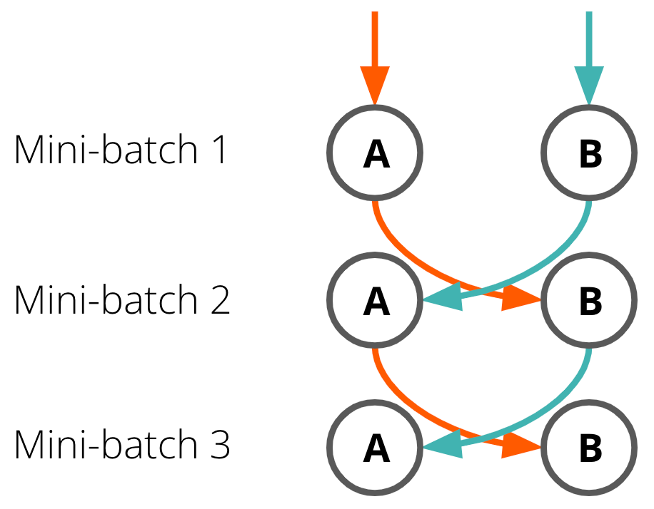
Figure 6. Exchange of training feed in co-teaching. Two peer networks exchange samples that are expected to be clean from noise. Image source: ⁷.

Co-teaching is one of the most popular and universal baselines in the domain of learning from noisy data. It has well-established empirical results, offers good performance even in extreme noise scenarios and can be simply integrated into almost any architecture or downstream task. Unfortunately, it also has a few downsides. Firstly, there is no theoretical guarantee that such a training setup will eventually converge. Secondly, we may end up with a consensus between the two networks, causing them to produce identical training feeds, and making the CT redundant.

Mixup

Mixup⁸ is a simple augmentation scheme that enforces linear behaviour of the model for in-between training samples (Figure 7). It linearly combines two training samples \((\pmb{x}_i, \pmb{y}_i)\) and \((\pmb{x}_j, \pmb{y}_j)\) with weight \(\lambda\) sampled from the Beta distribution. It results in a new augmented sample with mixed input features \(\pmb{x}_{aug}\) and a soft label \(\pmb{y}_{aug}\):

\[\pmb{x}_{aug} = \lambda \pmb{x}_i + (1 - \lambda)\pmb{x}_j \\ \pmb{y}_{aug} = \lambda \pmb{y}_i + (1 - \lambda)\pmb{y}_j \\\]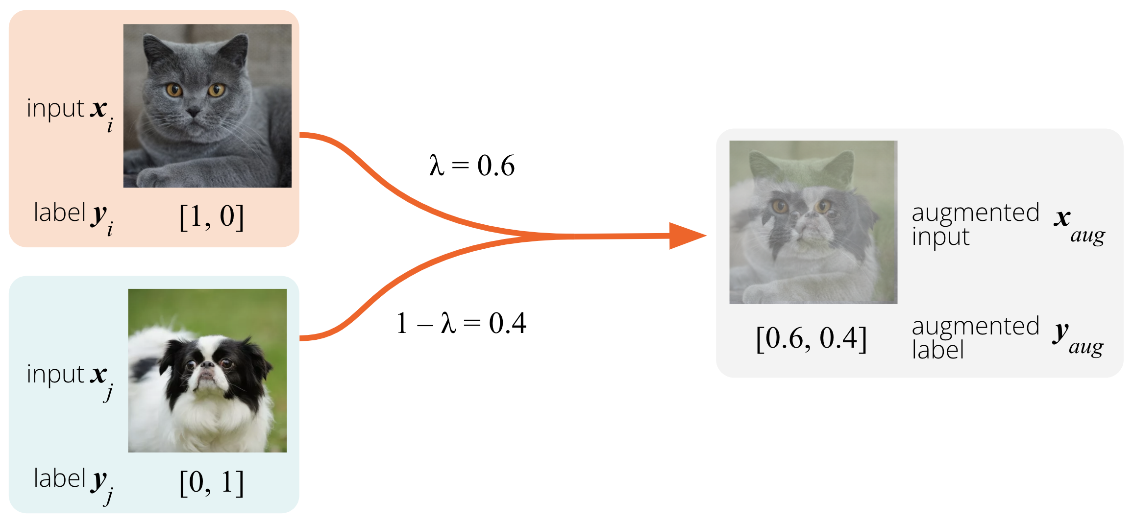

Figure 7. Augmentation through mixup. Two samples \(i\) and \(j\) are linearly combined into a synthetic image \(\pmb{x}_{aug}\) and a soft label \(\pmb{y}_{aug}\). This new augmented input encourages the model to linearly interpolate the predictions between the original samples.

The method is a simple, universal, yet very effective approach. It yields good empirical results while adding no severe computational overhead.

Cleaning up Allegro

Every offer has its right place at Allegro, belonging to one out of over 23,000 categories. The category structure is a tree consisting of:

• the root (Allegro),
• up to 7 levels of intermediate nodes (departments, metacategories, etc.) — over 2,600 nodes in total,
• over 23,000 leaves.

Offers located in wrong categories are hard to find and hard to buy. As such, we need a way to properly assign offers to correct category leaves. To this end, our Machine Learning Research team has developed a category classifier for Allegro offers.

The model in question is a large language model pre-trained on the Allegro catalogue (see more in Do you speak Allegro?) and fine-tuned for offer classification. Specifically, the downstream task here is extreme text classification: each offer is represented by text (title) and is classified into over 23,000 categories — hence the word extreme.

Classification is particularly challenging for offers listed in ambiguous categories such as Other, Accessories, etc. These categories are broad and hard to navigate, as they contain a wide variety of products. Most of those products actually belong to some well-defined categories, but the merchant couldn’t find the right place for those offers at the time of their listing, because of the very rich taxonomy of the category tree. Consequently, we decided to clean up the offers in ambiguous categories.

Here’s the setup (Figure 8):

• We train the category classifier on offers in well-defined categories: the model learns what lies where at Allegro.
• Next, we run inference on offers in ambiguous categories: the model moves the offers to their right destination.

Note that this task is subject to domain shift: the assortment listed in these ambiguous categories may be harder to categorise than the regular assortment in other categories.

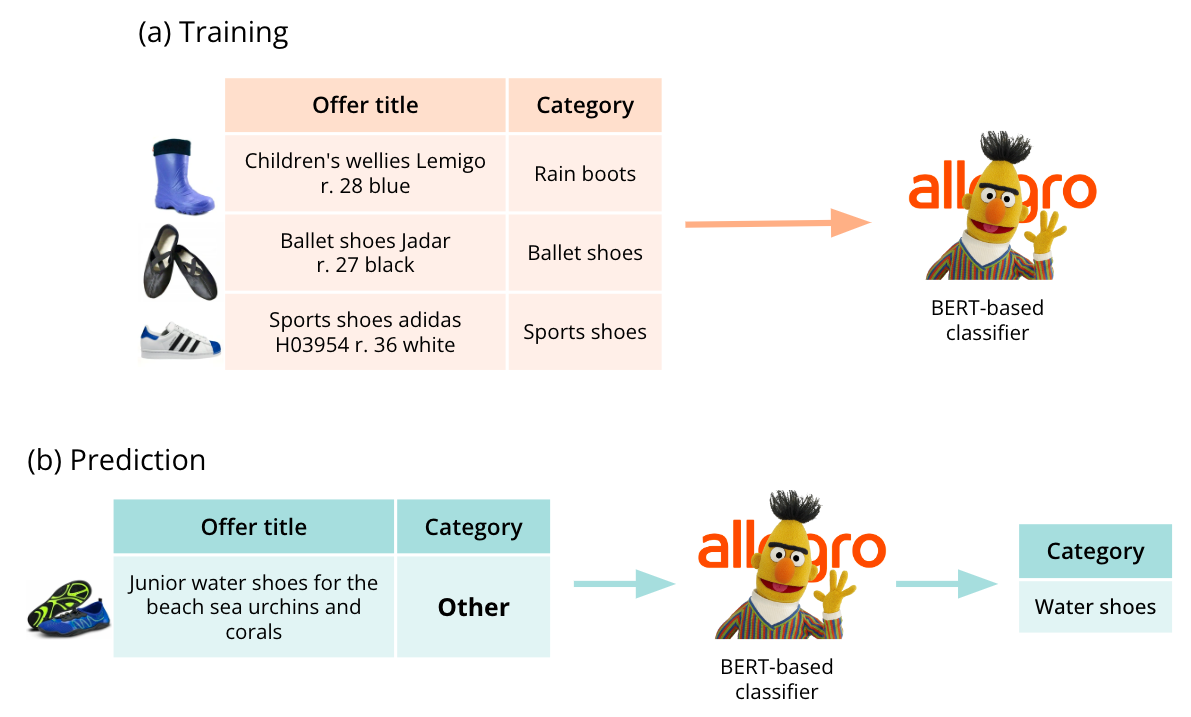
Figure 8. Category classifier: training & inference. The model is trained on offers listed in well-defined categories. Then, it is used to move offers from ambiguous categories (Other, Accessories, etc.) to the well-defined categories.

Real-world label noise at Allegro

The training set (offers in well-defined categories) is not 100% correct, for several reasons (Figure 9):

• the merchant may have put the offer in the wrong category,
• there are several similar categories in the catalogue,
• there is no appropriate category for a given offer,
• the taxonomy of the Allegro category tree changes over time.

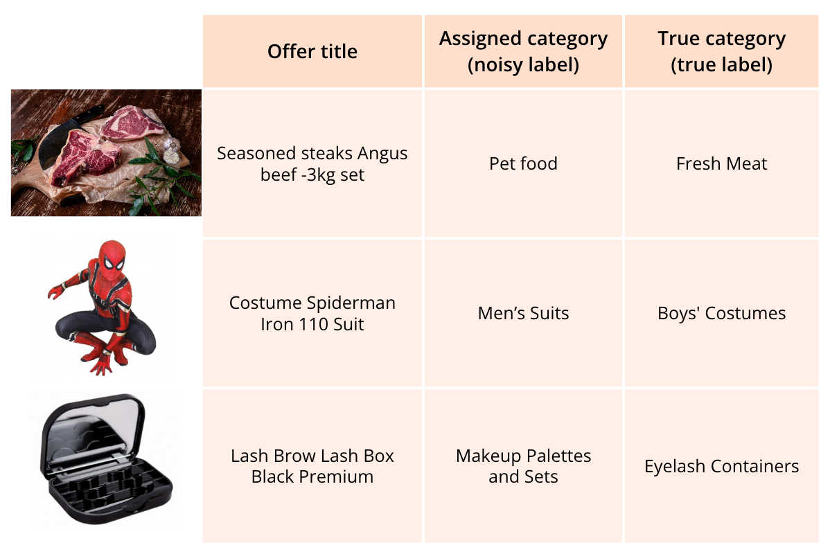
Figure 9. Examples of mislabelled offers. With over 23,000 categories at Allegro, listing each offer in its best-matching category can be challenging for merchants. Hence, label noise is an inherent feature of our training dataset.

The ML model is prone to memorisation of the wrong labels in the training set, i.e. overfitting. These errors will likely be reproduced at prediction time. Our goal is to train a robust classifier that will learn the true patterns and ignore the mislabelled training instances.

The training methods described in the previous section were developed and evaluated on computer vision tasks, e.g. image classification, into a relatively small number of categories. Here, we face the problem of extreme text classification. Thus, we need to adapt those methods for textual input and find out which concepts transfer well between the two domains.

Synthetic label noise

To evaluate the model’s robustness experimentally, we need to know a priori which training instances were mislabelled. For that, we use a generator of controllable noise. The experimental setup consists of five steps (Figure 10):

• dumping a clean dataset from a curated pool of offers that are certainly in the right place,
• splitting it into training, validation and test sets,
• application of synthetic noise to 20% of instances in the training and validation sets (changing the offer’s category to a wrong one),
• training the model on the noisy dataset,
• testing the model on a held-out fraction of the clean dataset.

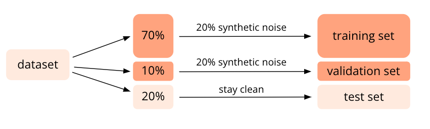
Figure 10. Testing the model’s robustness. The full dataset of clean instances (offers with true category labels) is split into training, validation and test sets. Next, label noise is introduced to the training and validation sets and the model is trained. The model is tested on a held-out fraction of the clean dataset.

This setup lets us answer the following question:

How much does the noise in the training set hurt the model’s performance on the clean test set?

This way, we can evaluate different methods of training classifiers under label noise and choose the most robust classifier, according to accuracy on the test set.

And… it works!

Below we present the results of experiments for 1.3M offers listed in the Construction Work & Equipment category. Symmetric noise was applied to 20% of the training set. This means that the category labels of that percentage of offers were changed to different randomly chosen labels. We evaluated the 7 training methods outlined above and compared them to the baseline: classification with cross-entropy loss.

Baseline: Memorising doesn’t pay off

How does the presence of noise impact the baseline model?

The validation curves for non-corrupted samples clearly show the severe impact of noisy labels on the model’s performance (Figure 11). In the early stage of training, the performance of the model trained on noisy data is on par with the metrics of the model trained on clean data. Yet, starting from the 4th epoch, the wrong labels in the noisy dataset appear to prevent the model from discovering the true patterns in the training data, resulting in a 5 p.p. drop in accuracy at the end of the training. We attribute this drop to the memorisation of the wrong labels: instead of refining the originally learnt concepts, the network starts to overfit to the noisy labels. The labels memorised for particular offers don’t help with classifying previously unseen offers at test time.

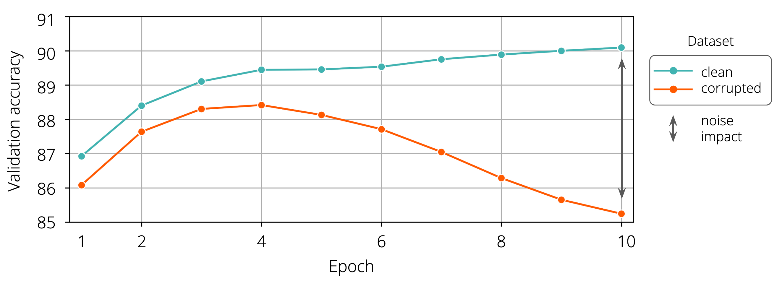
Figure 11. Degradation of the baseline model in the presence of noise. The 20% synthetic noise degrades the model throughout the training. In the end, the model trained on the corrupted dataset exhibits 5 p.p. lower accuracy in comparison to its clean counterpart

Towards robust classification

Does robustness imply underfitting?

To verify if the evaluated methods have any effect on the model’s performance when there is no noise in the training data, we tested all of them on a clean dataset without any synthetic noise.

In the absence of corrupted data, three of the tested methods (SPL, PRL and CT) are effectively reduced to the baseline Cross-Entropy. Therefore, the accuracy for those methods was exactly the same as for the baseline (Table 1). For mixup, the difference from the baseline was within the standard deviation range, so it was marked as no improvement as well.

For CCE and JSD the performance degraded, but only slightly — by 0.04 p.p. for the former and 0.34 p.p. for the latter. This drop is an acceptable compromise considering the robustness to noise that these methods enable (see below).

ELR was the only method that improved upon the baseline, by 0.07 p.p. As ELR relies on temporal ensembling, which diminishes the impact of corrupted samples during training, we hypothesise that our clean dataset contained a small number of mislabelled examples. Such paradoxes are a frequent case in machine learning practice, even for renowned benchmark datasets like CIFAR-100⁹.

Table 1. Test accuracy scores of the models trained on the clean and corrupted (20% synthetic noise) datasets for the 8 training methods. Light red highlight indicates deterioration in comparison to the baseline, while light blue denotes improvement. Notation: (mean \(\pm\) std)% from 5 independently seeded runs.

Method		Test accuracy [%]
		clean dataset	noisy dataset
Baseline		90.26 ± 0.03	85.31 ± 0.08
Robust loss function	Self-Paced Learning (SPL)	90.26 ± 0.03	88.51 ± 0.02
	Provably Robust Learning (PRL)	90.26 ± 0.03	88.31 ± 0.02
	Clipped Cross-Entropy (CCE)	90.22 ± 0.03	89.51 ± 0.01
	Early Learning Regularisation (ELR)	90.33 ± 0.01	89.29 ± 0.03
	Jensen-Shannon Divergence (JSD)	89.92 ± 0.02	89.24 ± 0.01
Implicit regularisation	Co-teaching (CT)	90.26 ± 0.03	88.72 ± 0.03
	Mixup	90.27 ± 0.02	86.02 ± 0.06

Robust classification results

All methods discussed in this study improved the model’s performance on the noisy dataset when compared to the baseline (Table 1). The best results were obtained with CCE (+4.2 p.p.), ELR (+3.98 p.p.) and JSD (+3.93 p.p.). CT, SPL, PRL performed a bit worse, but still proved to be quite robust, improving upon the baseline by 3.41 p.p., 3.2 p.p. and 3.0 p.p., respectively.

Mixup is a clear outlier — while it does improve upon the baseline by 0.71 p.p., this increase is noticeably smaller than for the other evaluated methods. Our interpretation is that the linear augmentation at the heart of this method regularises the DNN, but does not address label noise per se. Mixup treats all samples equally, even if their labels are corrupted. The marginal improvement upon the baseline is evident in the validation accuracy training curve (Figure 12). Mixup starts to overfit around the 5th epoch, similarly to the baseline, and unlike all the other methods.

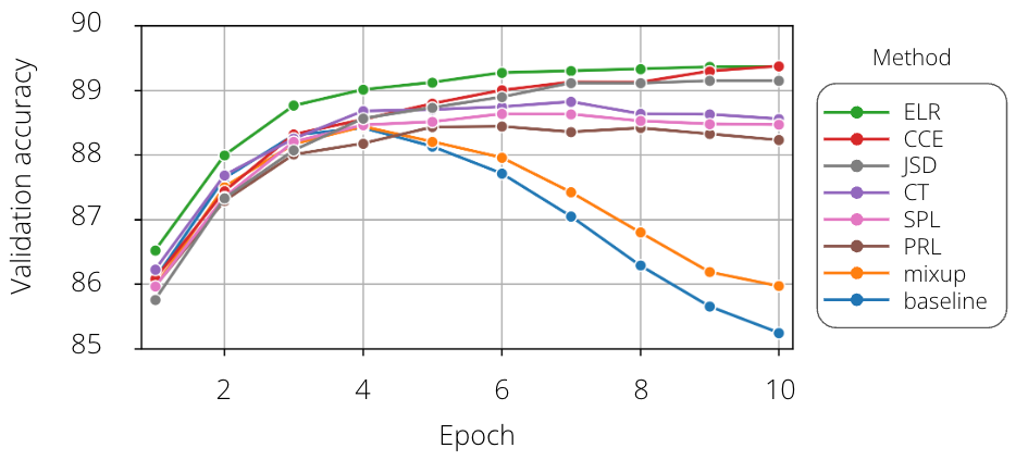
Figure 12. Validation accuracy during training. Validation accuracy for all methods was measured during training. It is evident that the best methods are CCE, ELR and JSD, with CT, PRL and SPL trailing slightly behind. Mixup behaves similarly to the baseline.

Conclusions

The problem of label noise is unavoidable in machine learning practice, and Allegro datasets are no exception. Fortunately, there exist numerous methods that diminish the impact of label noise on prediction performance by increasing the robustness of machine learning models. In our experiments we implemented 7 of those methods and showed that they increase prediction accuracy in the presence of 20% synthetic noise when compared to the baseline (Cross-Entropy loss), most of them by a significant margin. The simple Clipped Cross-Entropy proved to be the best, with an accuracy score of 89.51% (increase of 4.2 p.p. vs the baseline trained with noisy labels). This result is very close to the baseline trained with clean labels (90.26%). Thus, we showed that for the case of 20% synthetic label noise, it is possible to increase robustness so that the impact of label noise is negligible.

These experiments are only a first step in making classifiers at Allegro robust to label noise. The case of synthetic noise presented here is not very realistic: real-world label noise tends to be instance-dependent, i.e. it is influenced by individual sample features. As such, we plan to further evaluate the methods for increasing model robustness with a real-world dataset perturbed by instance-dependent noise.

If you’d like to know more about label noise and model robustness, please refer to the papers listed below.