


Turn-Based Offline Reinforcement Learning
This blogpost is the result of a research collaboration between the Allegro Machine Learning Research team and the Institute of Mathematics of the Polish Academy of Sciences (IMPAN), Warsaw.
Introduction #
Imagine the following scenario: you work in a company as a Research Engineer, and your manager is asking you to design a state-of-the-art algorithm to control a robot arm that should perform a critical task. You perform some research to find out that Reinforcement Learning (RL) would work really well in this case. However, you have the following limitations:
- The robot arm is built with poor hardware and can’t afford long and extensive usage.
- The robot arm can often be physically unavailable, and you may have access to it only for a limited period of time.
In addition to the aforementioned constraints, you also have another big problem: you don’t have any huge dataset containing past offline behavior of the robotic arm available. What can you do? Should you give up on applying RL to this problem? Is the problem even solvable with RL?
Don’t worry! We are here to help you! And to do so, we will walk you through the concept of “Turn-based Offline RL”. So let’s dive into it!
Standing between “Online RL” and “Offline RL” #
In Online RL, we normally have an agent that interacts with the environment, which is assumed to be always available. For each interaction, the agent will get a reward signal that assesses the quality of the action performed. The possibility of constant interaction with the environment marks the difference between the online and offline RL setting: in the latter, we break the environment-agent interaction loop, and we only have a buffer of transitions previously gathered using one or multiple unknown policies. Thus, in Offline RL, since there is no interaction with the environment, the buffer can be thought of as a static dataset that cannot be extended by any further exploration.
The idea behind “Turn-based Offline RL” falls exactly halfway between these two lines of thinking. Imagine yourself being able to build an initial static dataset filled with transitions generated by a random policy. Now that you have a static dataset, you can use it to train an agent using a preferred Offline RL algorithm. Then, suppose you have access to the target environment for a limited period of time. You have a (random) agent already trained! You can deploy it, interact with the environment, gather new experiences based on the policy learned so far, and enrich your static dataset. Now, having an updated (and better) dataset, you can re-train your Offline RL agent and repeat this process every time you are accessing the environment. Well, what we have described is exactly what we mean by “Turn-based Offline RL”. Let’s sum up the description in a few points:
- Start with a random policy and generate an initial static dataset.
- Train an agent using a preferred Offline RL algorithm using the dataset built in 1). We can call this phase “turn 0”.
- Access the environment the first time: collect transitions using the policy learned so far and extend the dataset with new data.
- Train your Offline RL agent again with a static dataset now composed of old (random) transitions and new (better) transitions (“turn 1”).
- Access the environment once again and collect new transitions.
- Train again your Offline agent (“turn 2”).
- Repeat the above steps as many “turns” as you can, i.e. as many times as you have the possibility to access the environment.
The main idea behind the turn-based procedure is that after each “turn” we will extend our dataset with “better” transitions, i.e transitions generated by more expert-like agents, and use Offline RL algorithms to train an even better (or at least similar) policy than the one used to generate those transitions. With the “Turn-based Offline RL” framework you can now see how you could possibly overcome the constraints for your hypothetical robot arm application: you could build a random dataset using some simulator; train an Offline RL agent with it; deploy the agent to interact with the robot arm for a limited period of time; extend the dataset with better data; re-train the agent, and repeat the process.
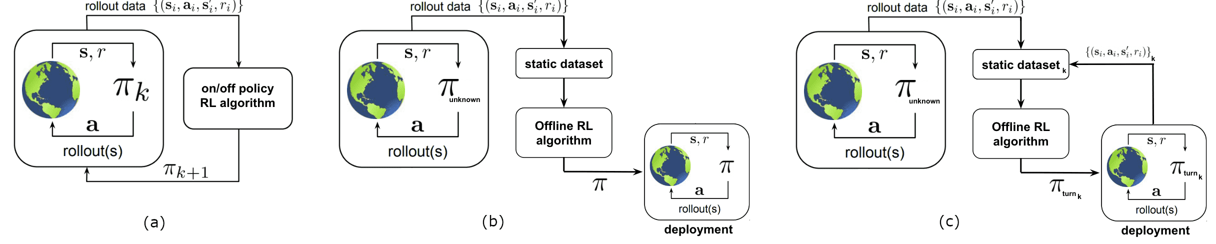 Fig.1 — Schematic comparison between Online RL (a), Offline RL (b), and Turn-Based Offline RL (c). For this diagram
we took inspiration from the paper Offline Reinforcement Learning: Tutorial, Review, and Perspectives on Open Problems
(Levine et al. 2020)
Fig.1 — Schematic comparison between Online RL (a), Offline RL (b), and Turn-Based Offline RL (c). For this diagram
we took inspiration from the paper Offline Reinforcement Learning: Tutorial, Review, and Perspectives on Open Problems
(Levine et al. 2020)
Turn-based Offline RL in practice #
In this blog post, we want to show you how you could make use of the “Turn-based Offline RL” framework to leverage the advances in Offline RL in applications where you could have the possibility of accessing the environment “in turns”. Fortunately, we don’t need any fancy robotic arm to do so! We have prepared for you a more comprehensive use case in order to explain the general idea behind it.
Experimental setup #
To showcase our idea, we are going to make use of a simplified environment. This tutorial will be in fact inspired by the NeurIPS 2020 Offline RL Tutorial Colab Exercise where the authors designed a simple GridWorld environment to test different ideas related to Offline RL.
GridWorld is a standard environment used in the RL community to test if algorithms can work in relatively easy situations or simply to debug them. In GridWorld, the agent starts at a starting point (“S”) and aims to reach a target point, sometimes called the reward (“R”) cell. The agent can either step up, down, left, or right, or stay still. Only empty cells can be stepped in, while non-empty cells, like the ones containing obstacles (walls), are not. The authors of the notebook provide an easy way to build such an environment from a string.
For the sake of this tutorial, we will work with a fixed 18x20 grid like the one specified by the string below. The “O” letter indicates empty spaces, “#” stands for walls, “S” is the starting state and “R” the target one. For clarity, we have drawn the grid for you.
grid = (
    'OOOOOOOOOOOOOOOOOOOO\\'
    'OOOOOOOOOOOOOOOOOOOO\\'
    'OOOOOOOOSOOOOOOOOOO#\\'
    'OOOOOOO##OOOOOOOOOO#\\'
    'OOOOOO#O#OOOOOOOOOOO\\'
    'OOOOOOOOOOO#OO#OOOOO\\'
    'OOOOOOOOOOOOOOOOOO#O\\'
    'OOOO#OOOOOOOOOOOOOOO\\'
    '##OOOOOOOO#OOOOOOOOO\\'
    'OOOOOOOOOOO#OOOOO#OO\\'
    'OOOOOOOOOOOOOOO####O\\'
    'OOOOOOOOOOOOOOOOOOOO\\'
    'OO#OOO#OOOOOO#OOOROO\\'
    'OOOOOO##OO#OOOOOOOOO\\'
    'OOO#OOOOOOOOOOOO##O#\\'
    'OOOOOOO#OOOOOOOOOOOO\\'
    'OOOOOOOOOOOOOOOOOOOO\\'
    '##OOOOO##OOOOOOOOOOO\\'
    'OOOOOOOOOOO#OOO#OOOO\\'
    'OOOO##OOOO#O#OOOOOOO\\'
)
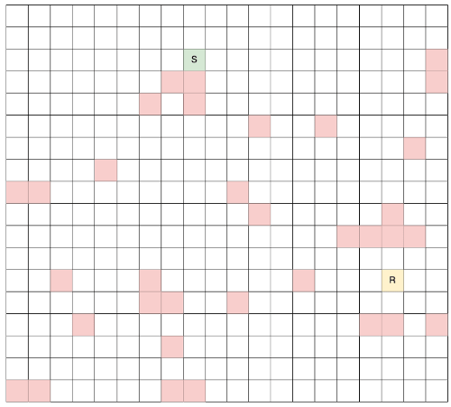 Fig.2 — The chosen grid for our experiments: the green cell (S) is the starting point; the
yellow cell (R) is the target point; white cells are empty while red cells contain walls.
Fig.2 — The chosen grid for our experiments: the green cell (S) is the starting point; the
yellow cell (R) is the target point; white cells are empty while red cells contain walls.
Please note that in our experiments we have tested different grid configurations and dimensions and we believe that the chosen dimensionality and obstacle distribution presented for this tutorial do represent a good experimental setup in order to arrive at reasonable conclusions. Indeed, the grid is small enough for the algorithm to be able to quickly iterate through different runs, and its configuration is complicated enough to lead to non-trivial results. In general, from our experience, things start to get interesting with grids NxM where N,M >= 12.
Agent’s visualizations #
In RL, it’s sometimes beneficial to visualize the policy your agents are learning. Since the environment we are playing with is relatively small, we can actually enumerate all possible state-action (s,a) pairs. When a specific algorithm runs, we are able to count how many times each of these pairs was visited, and we are able to visualize it as a heatmap, superimposed on the grid.
In our case, such heatmaps (that we call state-action visitation maps) can be really useful to understand, for example, the quality of a specific policy: a good state-action visitation map is created only by applying a good policy.
How would a map built using the optimal policy look like? Again, it’s a question we can answer only because we are in the ideal case of using a simple environment where we can know and do everything, like finding the optimal policy. We can use tabular Q-iteration to find an optimal solution for our case, hence producing the optimal state-action map that looks as follows:
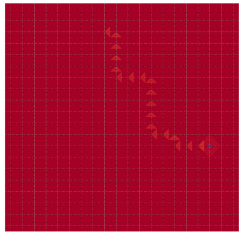 Fig.3 — State-action visitation heatmap generated by the optimal policy. Most of the time the agent reaches the target
cell in a few steps and then, it just stays idle without performing any further step.
Fig.3 — State-action visitation heatmap generated by the optimal policy. Most of the time the agent reaches the target
cell in a few steps and then, it just stays idle without performing any further step.
As you can see, in this case, almost every (s,a) pair has a value approaching zero, apart from the reward (“R”) state which has a big value. This is happening because once the agent knows the optimal policy, it will take very few steps for it to reach the target cell and once it’s reached, it will spend most of the time just waiting, without performing any further action. More precisely, the agent will spend the majority of the time in the (s,a) = (“R”, NOOP), where NOOP stands for “no operation”.
Let’s now visualize the heatmap generated by the uniform policy, i.e an agent that decides at random (with uniform probability) which action to take when being in a specific state. This approach would be the way to go in the majority of the cases and is the closest to the real case example. Suppose you don’t know anything about the environment you are going to interact with: the best you can do is to perform random exploration!
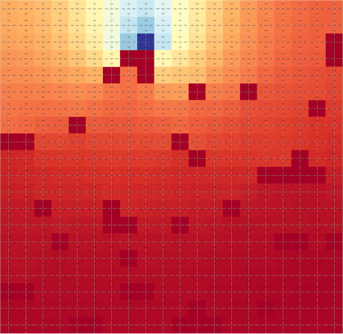 Fig.4 — State-action visitation heatmap generated by the random policy. The agent performs random exploration. As a
result of the random behaviour, cells in the surroundings of the initial state are visited on average more often than
further cells.
Fig.4 — State-action visitation heatmap generated by the random policy. The agent performs random exploration. As a
result of the random behaviour, cells in the surroundings of the initial state are visited on average more often than
further cells.
Since we start from the “S” cell at every episode, we have the highest probability of visiting the “S” state and all its surroundings. As we go further from it, the agent will start to pick different states depending on the run, and thus values on farther cells start to normalize and approach 0.0.
In the following, we will describe the algorithm in detail, and we will make use of these visualizations to understand if the turn-based approach is beneficial for learning a good policy when starting from a random one.
Algorithm #
Now let’s dive into the algorithm itself. Recalling the steps indicated in the previous section, we can describe the turn-based learning algorithm with the following pythonic pseudocode:
def run_turn_based_algorithm(init_policy,
                             num_turns,
                             num_seeds,
                             dataset_size,
                             num_iters):
    offline_dataset = []
    current_policy = init_policy
    num_of_trajectories_per_turn = dataset_size / num_turns

    for turn in range(num_turns):
        runs = []
        for seed in range(num_seeds):
            temp_dataset = offline_dataset.copy()
            trajectories_from_new_policy = deploy_and_sample(current_policy, num_of_trajectories_per_turn)
            temp_dataset.extend(trajectories_from_new_policy)
            policy, performances = run_offline_rl_algorithm(temp_dataset, num_iters)
            runs.append((policy, performances, trajectories_from_new_policy))

        best_policy, best_trajectories = find_best_run(runs)
        current_policy = best_policy
        offline_dataset.extend(best_trajectories)
Let’s explain each step involved in the algorithm. First, let’s define what the main parameters expected by the algorithm are:
init_policy— it’s the starting policy, most likely the random policy.num_turns— this is simply the total number of turns for which you will run the algorithm.num_seeds— if you work in RL you will be familiar with this argument: RL algorithms (and especially Offline RL ones) present large variability in the results due to their stochastic nature. That’s why instead of having one single run of the Offline RL algorithm, we will have several of them. For each run, we will produce the best policy and the best “new set of trajectories” to be used later in the algorithm (more on this step in the following).num_iters— this is simply the number of iterations we will run our Offline RL algorithm.dataset_size— as a design choice, we assume that the final dataset size has been fixed beforehand, as we do with the number of turns. However, both of these two conditions could be relaxed and one could run the algorithm as many turns as needed, getting a final offline dataset with an undefined size. However, please remember that in the real scenario you will probably not have the privilege of accessing the environment so often! You must do your best with a reasonable number of turns!
Now, following the logic of the pseudo-code, let’s describe the algorithm:
- Initially, we don’t have any transitions to train our Offline RL algorithm, so we initialize our
offline_datasetas an empty list. - We also initialize
current_policywithinit_policy, which most likely will be the random policy (an agent that has previously interacted with the environment taking actions uniformly at random). - Now, for each turn we run
num_seedstimes the following procedure:- We create a copy of
offline_dataset(temp_dataset) to train the current agent with the dataset collected so far. - We deploy the agent to the environment, in order to generate a new set of transitions using the current policy
(
trajectories_from_new_policy). - We extend the temporary dataset by
trajectories_from_new_policyand train an agent with it, using the preferred Offline RL algorithm and getting its correspondingpolicyandperformances. - We append the results to
runslist. - Once we have collected all the results, we pick the best policy and best-generated trajectories
out of the pool of runs (
find_best_run). - The
best_policyis now ourcurrent_policythat will be used for the next turn. - The
best_trajectorieswill are appended tooffline_datasetthat will is going to be used for the next turn.
- We create a copy of
- We repeat this procedure until we are satisfied with the performance or as many times (turns) we are able to access the environment.
Now, hoping the algorithm is clear to you, we need to answer two important questions.
Which Offline RL algorithm should be run? Actually here the choice is yours! In our case, we opted for using Conservative Q-Learning (CQL). Any algorithm may have its pros and cons. In our case we find it hard to set the CQL global parameters only once to be good for all the runs. What is happening is that initially our dataset will be full of random transitions, but as long as you proceed in turns, it will become richer in “more-expert” transitions. Thus, parameters like alpha for the CQL loss should be somehow adjusted in time. While in this tutorial we did not investigate this aspect, we found that for this very simplistic environment even CQL with alpha = 0 (equivalent to offline Q iteration) would work sufficiently.
How to aggregate results in order to get a representative policy and dataset for the next turn? That’s a hard question. For the sake of this tutorial, we have opted for the simplest of the approaches: out of the N runs, we will pick the one that gave us the best results (in terms of average reward). However, please note that this may be too optimistic and could lead to unexpected behavior in production. A better approach would actually be the one that takes into account the “average policy”. But, to “average out” policies is not a trivial task. We discuss this aspect in detail in the final section.
Results #
Visualizing the agent “in turns” #
First, we ask ourselves the following question: does the agent learn “in turns”? We can check this by visualizing subsequent state-action visitation maps:
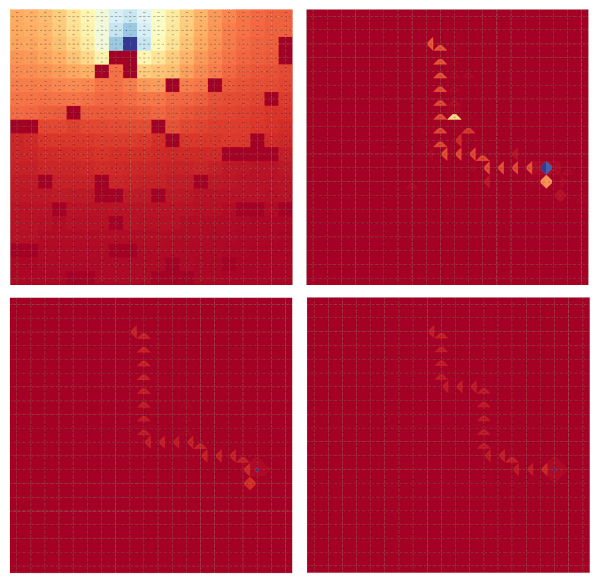 Fig.5 — Visualization of subsequent state-action visitation heatmaps. Here we visualize 4 subsequent turns — after one
single turn the agent learns the fastest path to reach the target cell. As long as we proceed in turns, the agent
improves its performance, eventually approaching a behaviour comparable to the optimal policy.
Fig.5 — Visualization of subsequent state-action visitation heatmaps. Here we visualize 4 subsequent turns — after one
single turn the agent learns the fastest path to reach the target cell. As long as we proceed in turns, the agent
improves its performance, eventually approaching a behaviour comparable to the optimal policy.
Our algorithm seems to work! When starting with a uniform policy, we can see that even after a single turn the agent quickly learns the fastest path to reach the target cell. As long as we proceed in turns, the model will consistently improve its performance, by quickly getting to the “R” cell even more often. In this sense, visitation maps get closer to the optimal one where the agent basically reaches the target in a few steps and then just stays there, without performing any further steps.
Does the agent improve its performance over time? #
How many turns are needed to start having results comparable to the optimal policy? In other words, how much better are we performing if compared to not doing any turn at all?
Let’s analyze the plot below. In this figure we are plotting the algorithm’s performance, measured in “averaged reward” (the higher, the better), as the amount of data available offline increases. In general, we expect the curve obtained by running the optimal policy (violet curve) to represent an upper bound: it’s the best we can achieve! On the other hand, we expect the curve obtained by running the random policy without any “turn” (green curve), to be our lower bound. Also, generally speaking, we expect that the more offline data is available, the better the achieved scores will be, since our chosen Offline RL will have more data coverage and possibility to converge to the optimal policy. Given this, we can observe that the performance of the turn-based procedure falls in the middle between the aforementioned upper and lower bounds: as the number of turns increases, the closer we get to the upper bound. However, we can observe that 3 turns are already enough to start having better performance than the lower bound. This plot confirms our hypothesis: “Turn-based Offline RL” stands exactly between Online RL (upper bound) and Offline RL (lower bound).
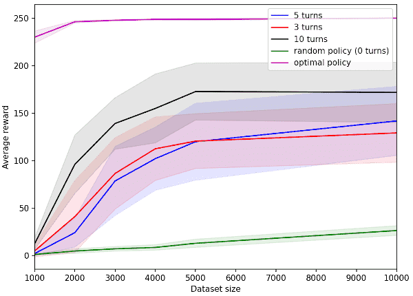 Fig.6 — This plot shows the comparison between baselines and the turn-based procedure in terms of average reward (the higher,
the better) as the size of the collected data used to train the algorithm offline grows. To obtain this figure,
we have run each of the algorithms for 30 seeds. For the optimal policy we run Q-iteration, while for the rest we
applied CQL with fixed alpha=0. For each run, CQL was fitted for 300 iterations.
Fig.6 — This plot shows the comparison between baselines and the turn-based procedure in terms of average reward (the higher,
the better) as the size of the collected data used to train the algorithm offline grows. To obtain this figure,
we have run each of the algorithms for 30 seeds. For the optimal policy we run Q-iteration, while for the rest we
applied CQL with fixed alpha=0. For each run, CQL was fitted for 300 iterations.
Conclusions and Future Work #
In this blog post we have presented a practical approach you could use to address cases where you have temporary and limited access to an environment, and you have computational resources at your disposal to train your RL algorithm “offline” only.
In fact, the proposed solution falls halfway between Online RL and Offline RL: our agent is warmed up by training it via Offline RL on a dataset generated by running the uniform random policy and then subsequently improved by accessing the environment in “turns”, thus partially simulating what you would get on a standard online RL scenario.
In particular, we show that:
- The turn-based procedure is effective since the policy learned in subsequent turns consistently improves as turns increase, matching the expectations. This result is demonstrated through some visualizations, showing how the agent chooses a better and faster path to target turn after turn.
- The turn-based procedure allows getting an agent that is better than a random one, even after a small number of turns. The performance of the turn-based agent will be upper-bounded by the performance of the optimal policy.
Moreover, we provide an easy-to-understand framework to prove the aforementioned hypothesis.
Finally, we want to point out some limitations of our work that could be addressed as future work:
- From one turn to the other, we pick the “best policy” as the one that achieves the best performance between all the runs via the “max” operator. This single policy is then propagated through the algorithm and used to generate the best new extension of the dataset. The inherent limitation of this approach is that by using the “max” we are not robust to the noise and we do not account for fluctuations in the performance of the Offline RL algorithm. A better approach would be aggregating policies by doing, for example, an ensemble of policies, and using this as the selected policy that is propagated forward in the algorithm.
- Running a fixed Offline RL algorithm on a dataset that keeps changing its distribution of states and actions in time could be really challenging since a lot of algorithms in the literature require accurate hypertuning of the parameters. In future work, we would like to address this problem, proposing, for example, a way one could compute new hyper-parameters using the dataset size and some other properties as parameters for the computation.
- One could argue that our hypothesis can work only on simplistic environments like GridWorlds. Even though we tested different configurations of grids, stressing more or less the algorithms, we admit that a more complete work would require the re-visitation of our hypothesis on a more diverse suite of environments. We plan to investigate this in the future.