Splitting data that does not fit on one machine using data partitioning
The following article is an excerpt from Software Mistakes and Trade-offs book. In real-world big data applications, the amount of data that we need to store and process can be often counted in the hundreds of terabytes or petabytes. It is not feasible to store such an amount of data on one physical node. We need a way to split that data into N data nodes.
The technique for splitting the data is called data partitioning. There are a lot of techniques to partition your data.
For online processing sources (like a database), you may pick some ID, for example, user-ID, and store a range of users on a dedicated node. For example, assuming that you have 1000 user IDs and 5 data nodes, the first node can store IDs from 0 to 200, the second node can store data from 201 to 400, and so on. When picking the partitioning scheme, you need to be careful not to introduce the data skew. Such a situation can occur when most of the data is produced by one or a group of IDs that belongs to the same data node. For example, let’s assume that the user ID 10 is responsible for 80% of our traffic and generates 80% of the data. Therefore, it will mean that 80% of the data is stored on the first data node, and our partitioning will not be optimal. In the worst case, this user’s amount of data may be too big to store on the given data node. It is important to note that for online processing, the partitioning is optimized for reading or writing data access patterns.
Offline big data partitioning #
We will focus now on the offline, big data processing partitioning.
For Big Data systems, we often need to store the historical data (cold data) for an “indefinite” amount of time. It is crucial to store the data for as long as we can. When the data is produced, we may not be aware of the business value that it can bring in the future. For example, we may save all user’s request data with all the HTTP headers. When the data is saved, there may be no use case for these HTTP headers. In the future, however, we may decide to build a tool that profiles our users by the type of device (Android, iOS) that they use. Such information is propagated in the HTTP headers. We can execute our new profiling logic based on the historical data because we stored it in the raw data. It is important to note here that the data was not needed for a long period.
On the other hand, we needed to store a lot of information and save it for later. Thus, our storage needs to contain a lot of data stored in cold storage. In Big Data applications, it often means that data is saved to a Hadoop distributed file system (HDFS). It also means that the data should be partitioned in a fairly generic way. We cannot optimize for read patterns because we cannot anticipate how those read patterns will look like.
Because of these reasons, the most often used data partitioning scheme for big data offline processing is based on dates. Let’s assume that we have a system that saves user’s data on the /users file system path and clickstream data in the /clicks file system path. We will analyze the first data set that stores the user’s data. We are assuming that the number of records that we store is equal to 10 billion. We started collecting the data in the year 2017, and it’s been collected since then.
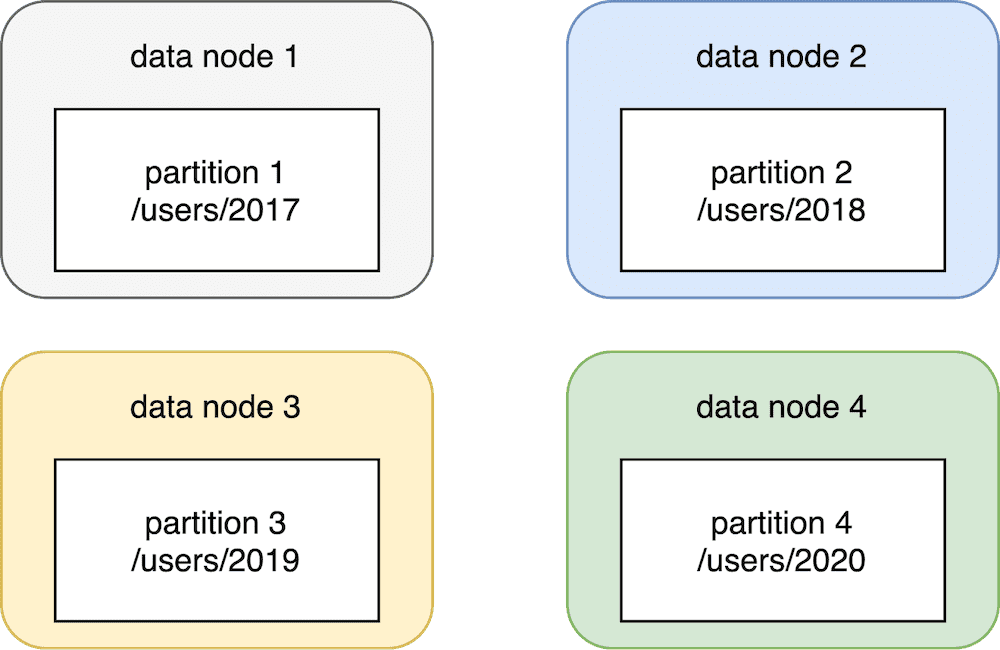
The partitioning scheme that we pick is based on the date. It means that our partition identifier starts with the year. We will have 2017, 2018, 2019, and 2020 partitions. If we would have smaller data requirements, partitioning by year may be enough. In such a scenario, the file system path for our user’s data would be /users/2017, /users/2018, and so on. It will be analogical for clicks: /clicks/2017, /clicks/2018, and so on.

Four data partitions #
By using this partitioning, the user’s data will have 4 partitions. It means that we can split the data into up to four physical data nodes. The first node will store the data for the year 2017, the second node for 2018, etc. Nothing prevents us from keeping all of those partitions on the same physical node when having four partitions. We may be ok with storing the data on one physical node as long as we have enough disk space. Once the disk space runs out, we can create a new physical node and move some of the partitions to the new node.
In practice, such a partitioning scheme is too coarse-grained. Having one big partition for all year’s data is hard from both a read and write perspective. When you read such data and are interested only in events from a particular date, you need to scan the whole year’s data. It’s very inefficient and time-consuming. It is also problematic from the writing perspective because if your disk space runs out, there is no easy way to split the data further. You won’t be able to perform a successful write.
Because of that reason, offline big data systems tend to partition the data in a more fine-grained fashion. The data is partitioned by year, month, and even day. For example, if you are writing data for the 2nd of January 2020, you will save the event into a /users/2020/01/02 partition. Such a partitioning gives you a lot of flexibility at the read side as well. If you wish to analyze events for a specific day, you can directly read the data from the partition. If you want to perform some higher-level analysis, for example, analyze the whole month’s data, you can read all partitions within a given month. The same pattern applies if you want to analyze a whole year’s data.
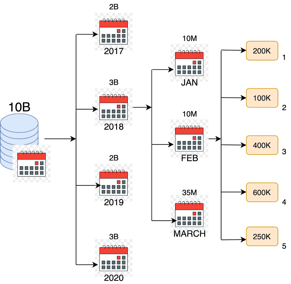
To sum up, our 10 billion records will be partitioned in the following way:

Date based data partitioning #
You can see that the initial 10 billion records are partitioned into year/month, and finally, a specific date of the month. In the end, each day’s partition contains a hundred thousand records. Such an amount of data can easily fit into one machine disk space. It also means that we have 365/366 partitions per year. The upper number of data nodes on which we can partition the data is equal to the number of days * the number of years we store data. If your one-day data does not fit into one machine disk space, you can easily partition your data further by hours of the day, minutes, seconds, and so on.
Partitioning vs sharding #
Assuming that we have our data partitioned by the date, we can split that data into multiple nodes. In such a scenario, we are putting a subset of all partition keys in a physical node.
Our user’s data is partitioned into N partitions (logical shards). Let’s assume that our partition granularity is a month. In that case, the data for the year 2020 has 12 partitions that can be split horizontally into N physical nodes (physical shards). It is important to note that N is less than or equal to 12. In other words, the maximum level of physical shards is 12. This architecture pattern is called sharding.
Let’s assume that we have three physical nodes. In that case, we can say that our user’s data for the year 2020 is partitioned into 12 partitions. Next, they are assigned to 3 shards (nodes). Each of the nodes stores 4 partitions for 2020 (12 partitions / 3 nodes = 4 partitions/node).

In our diagram, the physical shard is the same as the physical node. The partition keys (logical shards) are distributed evenly to physical shards. In case a new node is added to a cluster, each physical shard needs to re-assign one of its logical shards to a new physical node.
There are a variety of algorithms for shards assignments. They also need to handle shards re-distribution in case of adding or removing a node (failure or scale down). This technique is used by most big data technologies and data stores such as HDFS, Cassandra, Kafka, Elastic, etc., and they vary depending on the implementation.
At this point, we know the basics of data partitioning. Next, we need to understand how the partitioning algorithms work in depth. This is essential to understand if we want to reason about the big data tools we are using to get business value. This is discussed at length in the book.
This is discussed at length in the book. You can purchase it with a special discount here using the code allegrotech35.

