Domino - financial forecasting in the age of global pandemic
Accurate forecasting is key for any successful business. It allows one to set realistic financial goals for the next quarters, evaluate impact of business decisions, and prepare adequate resources for what is coming.
Yet, many companies struggle with efficient and accurate revenue forecasting. For most of them the task still rests on the financial department’s shoulders, performing manual analyses in Excel, lacking data science know-how, and relying on a set of arbitrary assumptions concerning the future. This process is often inefficient and prone to error, making it hard to distinguish trend-based patterns from manual overrides. In the end, the forecasts often turn out to be inaccurate, but it is difficult to diagnose the source of divergence - was it the fault of the model itself, wrong business assumptions, or perhaps unusual circumstances.
In order to overcome this problem, we decided to develop an AI tool which would allow us to forecast Allegro’s GMV (Gross Merchandise Value) based on a set of business inputs defined by the financial team. The purpose of the tool was twofold: to create automatic, monthly forecasts, and to enable creating scenarios with different input values. Examples of such inputs would be the costs of online advertising or the number of users enrolled in the loyalty program (Allegro Smart!).
Disclaimer: analysis and graphs presented in article are based on artificial data
Approach #
We named our project domino after Marvel’s universe foreseer-heroine Domino, but the name reflects also how the model is executed.
The model works as a graph of dependencies where each element is either a cause or effect of other steps (in the technical nomenclature known as DAG). Let’s go through an artificial example. Below you can find a diagram of the model. In the training phase we need to provide historical data for every node in the graph, i.e. we need to know actual online advertising spending (PPC), important holidays, and actual number of paid and organic visits to be able to accurately model the relationship between these variables.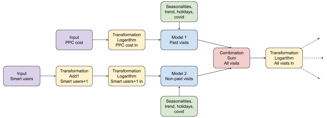
During the prediction phase, we only need actual data for violet nodes. These nodes usually represent our key business assumptions which are reflected in the company’s yearly budget. Next, our goal is to recreate all the succeeding values. Some of these subsequent steps will be just arithmetic operations like adding, summing, or applying logarithms (yellow and red). Other steps, here represented with blue nodes, may be Machine Learning models (e.g. Facebook’s Prophet). They can learn non-trivial effects like seasonalities, trends, holidays, and the influence of the preceding yellow nodes (i.e. explanatory variables).
You may wonder why we bothered with creation of such a complex graph of dependencies instead of making a single model taking all the business inputs as explanatory variables and returning future GMV values as the output. It’s what we want to model in the end, right? Why are we concerned with reconstructing the values of organic or paid traffic along the way? Well, we found out that following business logic yields much better results than inserting all the inputs into a huge single pot. Not only were the results less accurate in the latter case, but also the impact of explanatory variables on GMV was often not clearly distinguishable or even misleading. Instead, we recreated the business scheme by creating and training specialized models to reconstruct all the intermediate steps (e.g. predicting the number of paid visits) and merging their outputs with arithmetic operations or other models. However, remember that this approach comes at a cost! Using many steps in the modeling process may be both a blessing and a curse, since you need to train and maintain multiple models simultaneously.
One of the biggest advantages of this approach is that it allows us to capture very sophisticated non-linear relationships between inputs and the final target variable (GMV in our case). Following the business logic allows us to verify these non-trivial assumptions at each step.
Another advantage of this approach is that every model can be fitted separately with any model class you want. Having tested a few alternatives, we’ve chosen the Prophet library, but potentially any ML algorithm could be used (e.g. ARIMA, Gradient Boosting Trees, or Artificial Neural Networks).
A disadvantage is that the error in prediction propagates downstream the graph. So, if we make a mistake in a prediction in an early step, it will influence all the models and transformations dependent on it. The issue can be mitigated by creating accurate models at each step of the process.
Another slight disadvantage is that our Domino of models is not intrinsically interpretable (as most of the modern model classes). You have to use some post hoc methods to gather information on how the model does process data.
Technical implementation #
To develop and iterate over the DAG-type model we had to implement a custom Python framework. It allows for training and running models as well as arithmetic transformations in a predefined order.
The implementation allows us to utilize various model frameworks like Facebook’s Prophet, any Scikit-learn’s regressor, or an Artificial NN. For operational purposes, MAPE (Mean Absolute Percentage Error) can be easily calculated for each model in the graph, as well as for the whole DAG (again, the errors propagate downstream).
Below you can see how the above DAG can be implemented.
from domino.pipeline import Pipeline, Model, Transformer, Combinator
from fbprophet import Prophet

dag = Pipeline(input_list=['ppc_cost', 'smart_users'])

dag.add_step(step=Transformer(base_var='ppc_cost',
                             target_variable='ppc_cost_ln',
                             operation_name='ln'),
             step_name='transformer1')

dag.add_step(step=Transformer(base_var='smart_users',
                             target_variable='smart_users_add1',
                             operation_name='add1'),
             step_name='transformer2')

dag.add_step(step=Transformer(base_var='smart_users_add1',
                             target_variable='smart_users_add1_ln',
                             operation_name='ln'),
             step_name='transformer3')

dag.add_step(step=Model(model=Prophet(),
                  target_variable='paid_visits',
                  explanatory_variables=['ppc_cost_ln']),
         step_name='model1')

dag.add_step(step=Model(model=Prophet(),
                  target_variable='non_paid_visits',
                  explanatory_variables=['smart_users_add1_ln']),
             step_name='model2')

dag.add_step(step=Combinator(base_var1='paid_visits',
                            base_var2='non_paid_visits',
                            target_variable='all_visits',
                            operation_name='add'),
             step_name='combination')
Now we can use the dag object as a single model.
dag.fit(df_train)
predictions = dag.predict(df_test)
To understand what’s happening inside the DAG, we implemented two methods of calculating MAPE on every step:
dag.calculate_mape_for_models(x=df_test)
dag.calculate_mape_for_dag(x=df_test)
They both return dictionaries of model-MAPE pairs. The calculate_mape_for_model method checks each model separately, and calculate_mape_for_dag takes into account the errors propagating from preceding steps. These are examples of results:
models_mape = {
   'transformer1': 0.0,
   'transformer2': 0.0,
   'transformer3': 0.0,
   'model1': 0.1,
   'model2': 0.05,
   'combination': 0.0
}

dag_mape = {
   'transformer1': 0.0,
   'transformer2': 0.0,
   'transformer3': 0.0,
   'model1': 0.1,
   'model2': 0.05,
   'combination': 0.09
}
Note that the combination step has MAPE equal to zero in models_mape and a positive one in dag_mape. That’s because it does not generate any error, as it’s an arithmetic operation, but it can propagate errors from previous steps.
Last but not least, there is an explainability method calculate_variable_impact that helps to evaluate how changes in initial inputs impact the subsequent steps in the graph. For example, we can check what is going to happen if we decrease PPC costs by 10% and increase the number of Smart users by 5%.
dag.calculate_variable_impact(x=df_test,
                              variables_list=['ppc_cost', 'smart_users'],
                              variables_multiplier_list=[0.9, 1.05],
                              diff_type='relative')
The percent change will be calculated on every node, i.e. smart_users_add1_ln, paid_visits, and all_visits. We will be able to evaluate how such changes affect not only the GMV, but also all intermediary KPIs.
Facebook’s Prophet #
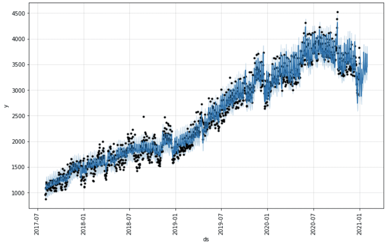
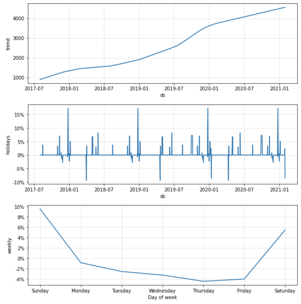
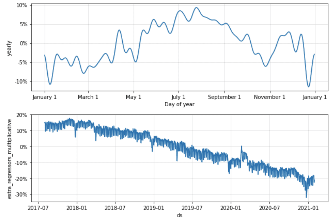
Having tested various modelling techniques, we chose the forecasting procedure offered by Facebook’s Prophet library (https://facebook.github.io/prophet/). It uses a decomposable Bayesian time series model with three main components: seasonalities, trends and errors, hence it works well for our time series that have strong seasonal effects. Moreover, the Prophet model is robust to outliers and shifts in the trend, which proved very useful in some models. Mostly, however, we assumed the trend to be flat. The piecewise linear trend explains some of the variance of the dependent variable which could otherwise be explained by the regressor variables/inputs. Given that the purpose of the tool is to allow testing scenarios with different values of the inputs, we needed our models to estimate the relationship between the explanatory variables and the dependent variable, but accounting for seasonality, holidays and some external events (e.g. COVID) only. The graphs below show an example of the forecast components generated by the Prophet, with linear trend, effect of holidays, weekly and yearly seasonality, as well as effect of explanatory variables.
Adding our domain knowledge about the analysed time series (e.g. calendar effects) and possibility of tuning the parameters of the model (e.g. the strength of the weekly seasonality effect) makes Prophet a perfect fit for our purpose.
Modelling framework #
Both the patterns and relationships between the variables change slightly over time, hence it would be naive to expect that once all the models are tuned they will give best forecasts forever. It is therefore necessary to analyze the results every time the forecasts are made (every month) and apply necessary tweaks to the models.
As in every machine learning project, we split our time series into:
-
Training dataset: the actual dataset that we use to train the model, i.e. the model learns from this data.
-
Validation dataset: the sample of data used to provide an unbiased evaluation of a model fit on the training dataset while tuning model hyperparameters; in time series, this is a time period following the training dataset time series.
-
Test dataset: the sample of data used to provide an unbiased evaluation of a final model fit on the training dataset. In time series, this is a time period following the validation dataset time series.
The COVID-19 pandemic wreaked havoc on our time series, not only changing the patterns temporarily, but often introducing shifts in the trend. Given that we worked on the tool during summer 2020, we were forced to use quite a non-standard approach to hyperparameter tuning and model testing (e.g. to maximize the length of the training period, so that it includes at least a month of the data showing post-COVID comeback to a new normal).
In the long run, we expect that the process will stabilize and we’ll be able to conduct the following adjustment procedure each month: training all the models using the parameters set in the previous month, testing them on the last 2 months of observed data, evaluating monthly and daily MAPE. When forecast errors in GMV prediction or any intermediate model are too large, we scrutinize the graphs of observed vs forecasted values. It is also helpful to compare the predictions vs observed values for the same period of the previous year. This step allows us to verify whether there are any seasonalities or patterns that were not detected by the tuned model. We can fine-tune the models either manually, or using the automatic hyperparameter optimization framework.
-
Hyperparameter tuning using Optuna (https://optuna.org/), half a year’s worth of data and expanding window approach (see visualisation below). This means that we will fine-tune our models using 6 sets of validation datasets, each consisting of 1, 2, 3, 4, 5 and 6 months. The Optuna framework will suggest parameters that minimize the average of MAPE over these datasets.
-
Testing the tuned models on 2 last months of observed data, measuring MAPE on the forecasted vs observed values of GMV, as well as on all intermediate models.
-
If any of the MAPE is not satisfactory, again scrutinizing the graphs and fine-tuning the models manually.
Once we are satisfied with the results, we always check if the changes made to the models do not result in some explanatory variables having unexpected signs of impact on GMV.
Despite the changes in time series, we are expecting that in the long run fewer and fewer tweaks to the models will be necessary, and less work will be required from the analysts to maintain the tool.
User interface #
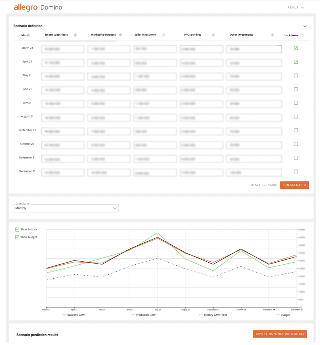
To make the model easily accessible by business users, an interactive application was prepared. The user has default inputs set for upcoming months. They can change their values and get model predictions by clicking the “RUN SCENARIO” button. The predictions can be seen in daily, weekly and monthly granularities. If the user chooses to, they can export the predictions in CSV format. You can find an anonymised print screen of the tool below.
Summary #
As a result of the project, we developed a solution providing incredible business value. The main features of the tool are:
-
Great forecast accuracy - we managed to get below 2% MAPE
-
Stability - the structure of the model remains the same and the inputs have the same impact direction over time
-
Responsiveness - the forecasts change with changes in the business inputs
-
Interpretation - though the model is not intrinsically interpretable, we developed methods to check how well it works
-
Interactive UI - stakeholders can experiment with various business scenarios online
Domino proved its effectiveness in hard and demanding times while giving us a lot of practical knowledge related to modeling of such a complex business metric. And, we already started using these lessons in new upcoming projects.


