

A/B testing good practice – calculating the required sample size
Developing our own A/B testing platform from scratch came with many lessons during the process. Our platform was built for people who differ vastly in terms of statistical knowledge, also for those who are not familiar with statistics at all. So the main challenge wasn’t technical implementation. The hardest thing was (and still is) developing good practices and spreading them among our users. We want to share some of our current knowledge that we think is crucial for A/B testing at scale. From this article, you will get to know about calculating sample size, what it means and what benefits it provides for you and your organization.
Quick reminder of the statistical significance #
If you are not familiar with the concept of statistical significance, we prepared a quick guide that will give you the required intuition to understand the whole article. If you are familiar with the concept, just skip this part.
Let’s suppose that you are conducting an experiment that checks if making the button larger increases its CTR (click-through rate). You want to deploy the larger button if it performs better than the smaller button in terms of the CTR. 50% of your users see the smaller button and 50% see the larger button.

After you stop your experiment, you check the CTR of each version of your button and you can see that the larger button has 10% CTR and the smaller button has 9% CTR. Is it proof that the larger button is better in terms of the CTR than the smaller button? Not really.
Let’s say that you run an A/A test. For example a small button vs small button. Even when you compare the same buttons, you will always see some difference between their CTR. So the question is: how do I know if the difference in CTR comes from the change that I test and not from random users’ behaviour?
The answer is: you need to calculate the statistical significance. To calculate the statistical significance for the described experiment you need the number of clicks and the number of views for each button. Let’s say that the large button got 100 clicks and 1000 views and the small button got 90 clicks and 1000 views. Using this calculator you get the result “Result not significant!”:
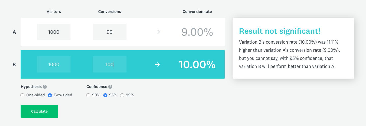
In other words, the difference in buttons CTR comes from random user behaviour and not from the actual difference between the buttons. Now, let’s modify the button performance a bit. Let’s say that the large button got 200 clicks and 1000 views and the small button got 90 clicks and 1000 views. When you calculate the significance again you get “Significant result!”:
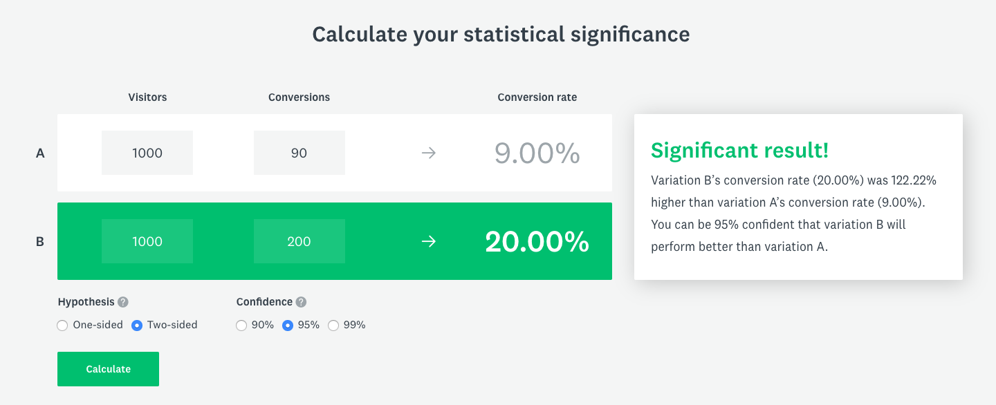
It means that the difference between the buttons CTR comes from the real difference between them and not from random users’ behaviour.
Unfortunately, the statistical significance is not a perfect tool and it sometimes gives you false results. Even when you see “Significant result!”, in reality, it can be “Result not significant!”. It works both ways. In conclusion, there are 4 possible results of the statistical significance test:
| “Significant result!” | “Result not significant!” | |
|---|---|---|
| In reality, there is no difference between the buttons’ CTR | false positive | true negative |
| In reality, there is a difference between the buttons’ CTR | true positive | false negative |
Let’s go through each option:
- false positive happens when the difference in buttons’ CTR comes from random user behavior but calculator says the opposite, that results are statistically significant. In that situation you deploy larger button because you think that it performs better but in reality there is no difference.
- true negative happens when the difference in buttons’ CTR comes from random user behaviour and calculator confirms that by showing “Result not significant!”. In that situation, you don’t deploy a larger button because there is no difference in CTR.
- true positive happens when the difference in buttons’ CTR comes from its characteristics and not just from random user behaviour and the statistical test admits that by giving the significant result. You deploy the larger button and that’s right choice.
- false negative happens when the reality is that difference in CTR comes from buttons characteristic but the statistical significance test says that it comes from random user behavior. In result you don’t deploy larger button because you think that difference came from random user behaviour. You just missed the opportunity!
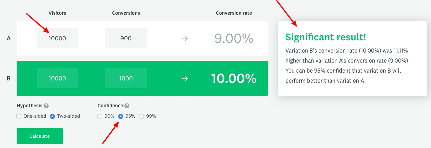
Ok, so now you know that the statistical significance test may be wrong. But what is the probability of getting the false result? The answer is: it depends. You can control the probability of getting false positives by setting confidence levels. Confidence level defines the probability of getting true positive results. It doesn’t mean that you can just set confidence level at 100%. Different confidence levels require different sample sizes. A higher confidence level demands more samples. That’s why you can’t just set the confidence level at 100%, because it requires an infinite number of samples. In the case of the example experiment, one button view is one sample.
As you can see, in the picture below, by increasing the number of samples, the non-significant result changed to significant result (percentage CTR values are the same as previous ones):
If you look closely at the results that calculator provides, you can see the details section. The details section contains information used by the calculator to determine the final result.
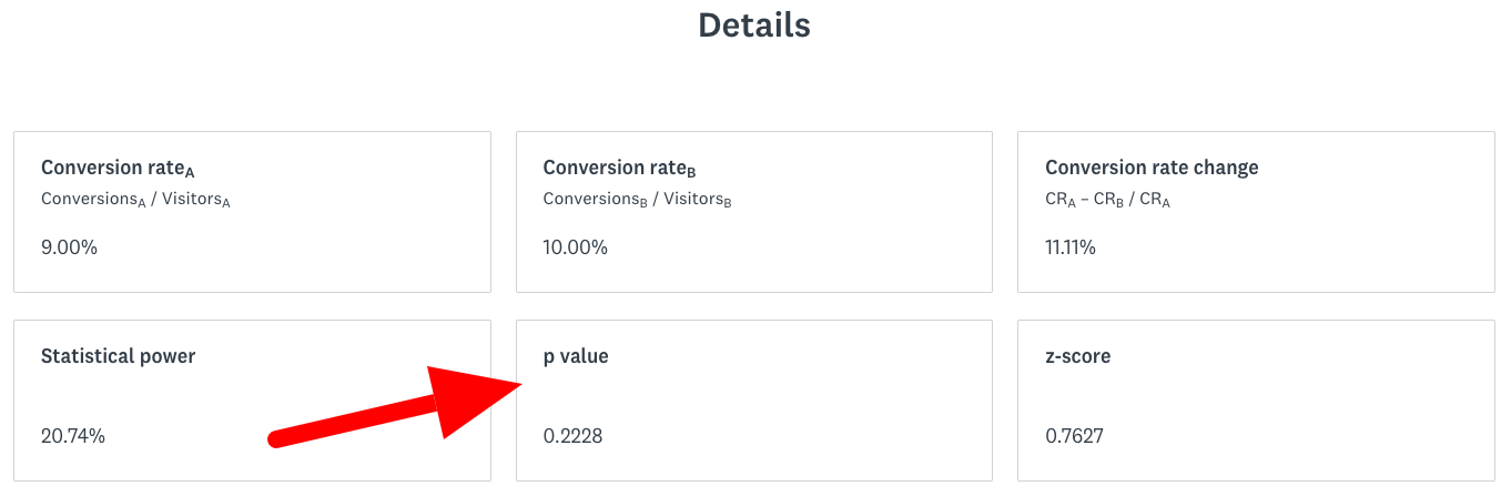
The key value used to determine the final result is the p-value. Under the hood, calculator calculates the p-value and compares it with the threshold calculated from the confidence level:
\begin{equation} \frac{ 100\% - \textrm{confidence} }{2} \geq \textrm{p-value} \end{equation}
If the p-value is above the threshold, the result is not significant.
What is the problem? #
The concept of statistical significance is generally hard to understand. We noticed that our users don’t fully understand it. Because of that, they often take an invalid approach to conduct tests. If you are aware of the concept of statistical significance and you are not calculating the required sample size already, it’s very likely that:
- You stop your test as soon as you see the statistical significance.
- You stop your test after a specific period, for example, 2 weeks.
In both cases, you lower your chances of conducting a successful test due to premature stop. The second option is much better than the first one, but still, it’s not perfect.
First of all, why is stopping the test after you see the first significant result a bad practice? It’s because your chance of getting false positive is rising. False positive occurs when we see a statistically significant difference where there is no such difference.

In that situation, you are very likely to deploy a change that has no real effect or has a negative effect. On Figure 1 you can see that after gathering 13 samples you could stop gathering them (because p-Value is smaller than 0.05 at that point) and mistakenly conclude that there is a statistically significant difference, where there is no difference.
The second option is a step in a good direction. Still, it’s not a perfect solution, because, for example, when you want to detect a 1% difference you need to gather more samples than when you want to detect a 10% difference. Two weeks might be enough to detect a 10% difference, but it might not detect a 1% difference. Problem is that the result of your test depends vastly on a number of samples. You can run a test for a year and still not gather enough samples to prove your hypothesis. You can see on Figure 2 that fraction of detected true positives (detecting a difference when there is one) is increasing with sample size.

Fortunately, there is a way to calculate the required sample size based on your hypothesis. Knowing the required sample size and daily traffic on your website you can calculate how long your test should last.
What are the benefits? #
A/B testing is time-consuming, no matter how powerful and convenient your tools are. Tests need to be designed, implemented, run on production and concluded. Each phase can cause making wrong decisions or wasting time. Calculating the required sample size means spending a little bit more time on test design. But it pays out by making inference easier and less error-prone.
One of our current goals in Allegro is to improve experimentation pace. There are obvious ways to improve it, for example reducing the number of implementation errors that cause repeating the whole test. Making a hypothesis more strict by calculating the required sample size is a more subtle change from a user perspective. But it causes positive changes in the whole platform by:
- Reducing the number of insignificant results caused by an insufficient number of samples.
- Forcing users to form a strict hypothesis.
- Saving time that could be lost because of running test too long.
Calculating the required sample size #
Depending on the type of metric that you want to change and on the test that will be run, you are going to use different methods to calculate the required sample size. Below, we described the algorithm of calculating the required sample size for most common metrics.
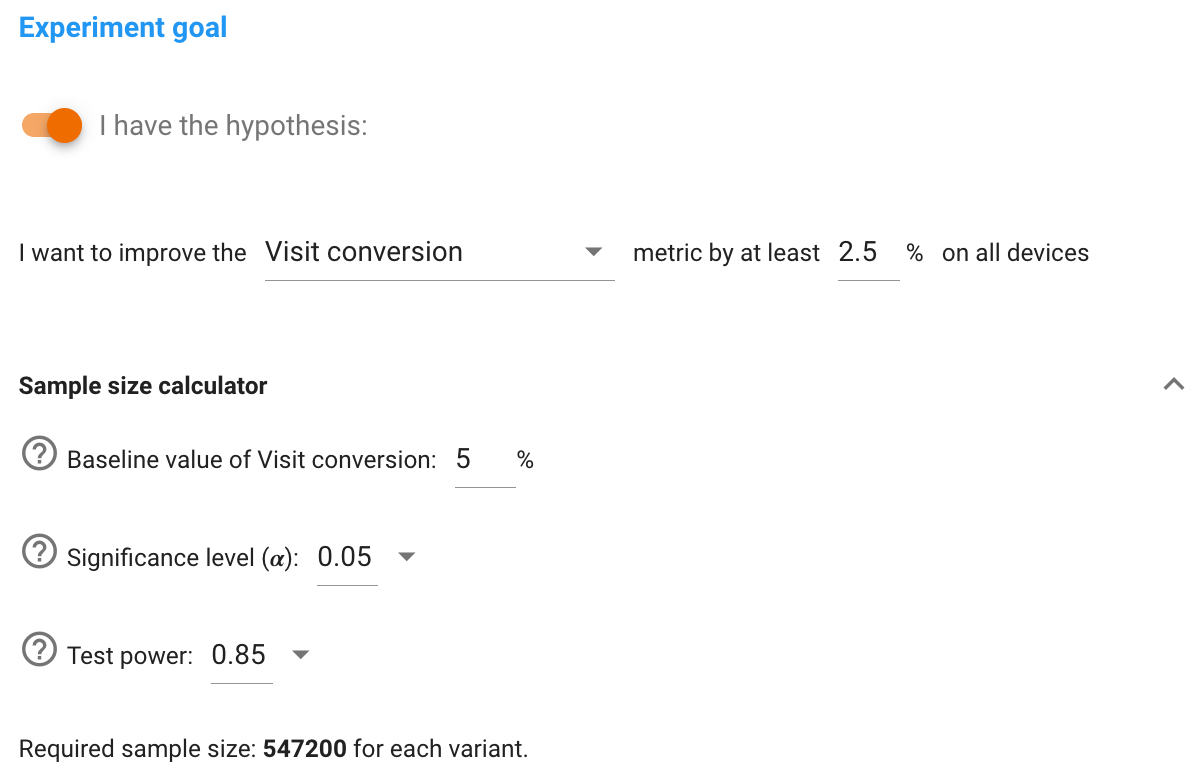
Using sample size calculator for binary metrics #
A binary metric is defined as the number of successes divided by the number of trials. Example binary metrics are conversion rate or CTR (click-through rate). In the case of CTR, a number of trials are how many times a user saw the element and number of successes is how many times a user clicked on the element.
Let’s say that you want to conduct an experiment that checks if changing the colour of the button from blue to red increases its CTR. We also know that the CTR of the blue button is 5%. First, you need to form the hypothesis, for example:
Changing the button colour from blue to red will increase it’s CTR by at least 10% from the current 5%.
That’s the most basic form of the hypothesis that you can use to calculate the required sample size. It contains three crucial elements:
- Which metric you want to change, in this case, it’s CTR.
- What is the minimal impact that you want to detect, in this case, it’s +10% (so in the tested variant it should be 5.5% or more).
- What is the base (current) value of the metric, in this case, it’s 5%.
You can use the Optimizely calculator to calculate the required sample size based on that hypothesis. The baseline conversion rate will be 5% and the minimum detectable effect will be 10%. For now, you can forget about the third parameter – statistical significance and use the defaults. The required sample size per variant should be 31,000.
When you know the required sample size per variant, you can combine that with information that is provided by your analytics to estimate how long your test should be active on production. Let’s say that the button is viewed 1000 times in a single day. Knowing that you can conclude that you should run your test for 62 days. This is so because when you split your users into the two equal-size groups, each generates 500 views per day. So to gather 31,000 samples per each group you need 31,000 / 500 = 62 days.
Finally, let’s go back to the third parameter – statistical significance. There is no way of completely avoiding a false positive outcome. Fortunately, you can control the probability of false positive by changing the value of the significance level. As a result, the sample size will naturally increase. Intuitively, by doing more trials you can be more sure about test outcome. That’s why when you increase statistical significance, the number of required samples is rising. For example, rising the statistical significance to 99% from the default 95% change the number of required samples from 31,000 to 33,000. Remember that what is called in this calculator statistical significance is formally named confidence level.
If you are interested in making your calculations more precise you need to know that there is the fourth parameter that is not included in Optimizely calculator - power. Power is the probability that the test will detect the real difference. Increasing the power will also result in an enlarged sample size. If you want to manipulate the test power, you need more complex calculator.
Calculating sample size for binary metrics (CTR, conversion rate, bounce rate, etc.) #
We implemented our own sample size calculator for our experimentation platform. Below, we describe the theory behind our calculator.
For binary metrics, we use the chi-squared test for independence to calculate a statistical significance of a difference between two variants. We use it to test the relationship between expected frequencies and observed frequencies in two categories and this is exactly what we want. To estimate sample size \(N\) we use the following formula (which assumes that sample sizes of both variants are equal):
\begin{equation} N = \frac{2(z_\alpha+z_{\beta} )^2 \mu(1-\mu)}{\mu^2 \cdot d^2} \end{equation}
where \(\alpha\) is confidence level and \(\beta\) is the test power. These \(z\)-values might look a little bit confusing, but don’t worry – they are tabulated values, which you can simply read from the \(z\)-score table. \(\mu\) is the base (current) value of the metric and \(d\) is the minimal impact that you want to detect. As you can see all of the parameters are known and you can calculate the estimated sample size.
Calculating sample size for non-binary metrics #
A non-binary metric is any metric that isn’t binary, as the name says. It could be for example AOV (average order value) or GMV (gross merchandise value). To test whether there is a statistically significant difference between two variants we use the nonparametric Mann-Whitney U test. This test can be used to determine whether two independent samples were selected from populations that have the same distribution. Calculating the sample size, in this case, is a bit more tricky. There is no online calculator to do that and here we propose our method of calculating sample size \(N\). The parametric equivalent of Mann-Whitney U test is Student’s t-test. It is known that the sample size for our nonparametric test is at most 15% bigger than the sample size that is required for the parametric version, so we calculate sample size for t-test and then multiply it by 1.15. Here is the formula:
\begin{equation} N = \frac{2(z_\alpha+z_{\beta} )^2 \sigma^2}{\mu^2 \cdot d^2} \cdot 1.15 \end{equation}
Just like previously \(\alpha\) is confidence level, \(\beta\) is the test power, \(d\) is the minimal impact that you want to detect, \(\mu\) is the base (current) value of the metric and \(\sigma\) is its standard deviation. Now you can easily calculate the estimated sample size of \(N\).
Summary #
When you run an experiment you should remember a couple of things that are related to statistics. First of all, you should state your hypothesis correctly. Secondly, you should remember about possible outcomes (false positive, false negative, true positive and true negative) of your experiment and their probabilities. Last but not least, calculate your desired sample size before running an experiment to avoid misinterpreting results. Especially, you shouldn’t stop an experiment just at the moment you see a statistically significant result. If you have problems with estimating sample size, there are several online calculators or you can use formulas provided by us.