Caching is a good and well-known technique used to increase application performance and decrease overall system load. Usually small or medium data sets, which are often read and rarely changed, are considered as a good candidate for caching. In this article we focus on determining optimal cache size based on big data techniques.

Background

Some numbers to understand the problem

Allegro is the largest e-commerce site in Central Europe. Every day you can browse and purchase one of 50 millions offers available on the site. To show so-called Allegro “listing” page, Solr is requested with user query for items’ identifiers, then items’ data are retrieved from Cassandra, which is super-fast, scalable, and reliable NoSQL database.

As a team responsible for listing reliability and performance, we started to look for a solution that decreases the load generated by our application on Cassandra. The first and obvious idea that appeared was to cache items in listing application. However, we didn’t want to build a distributed cache as it adds complexity to the system. Cassandra itself is very efficient.

Hypothesis — caching small fraction of items can save many requests

We thought about local cache as an opposite to distributed cache. But there are 50 millions of items, and they can’t fit into single application instance memory. Our intuition told us that caching only a small fraction of items could be a good solution because probably items are not requested at equal frequency. We didn’t want to implement our caching engine with random parameters’ setup blindly. Instead, we decided to use our internal Hadoop-Spark big data stack and Jupyter Notebooks to prove or debunk the hypothesis: “it is possible to significantly decrease traffic from listing application to Cassandra by caching only a small percent of listing items”.

Estimating the cache efficiency using big data

Whenever you search on Allegro by phrase or browse the category tree, the id of each found item is stored in Hadoop. So let’s get all ids found during last 24 hours.

We define:

• n as a number of finds,
• f(n) as a number of items which were found exactly n times.

For example, f(7) tells us how many items were found exactly 7 times in last 24 hours.

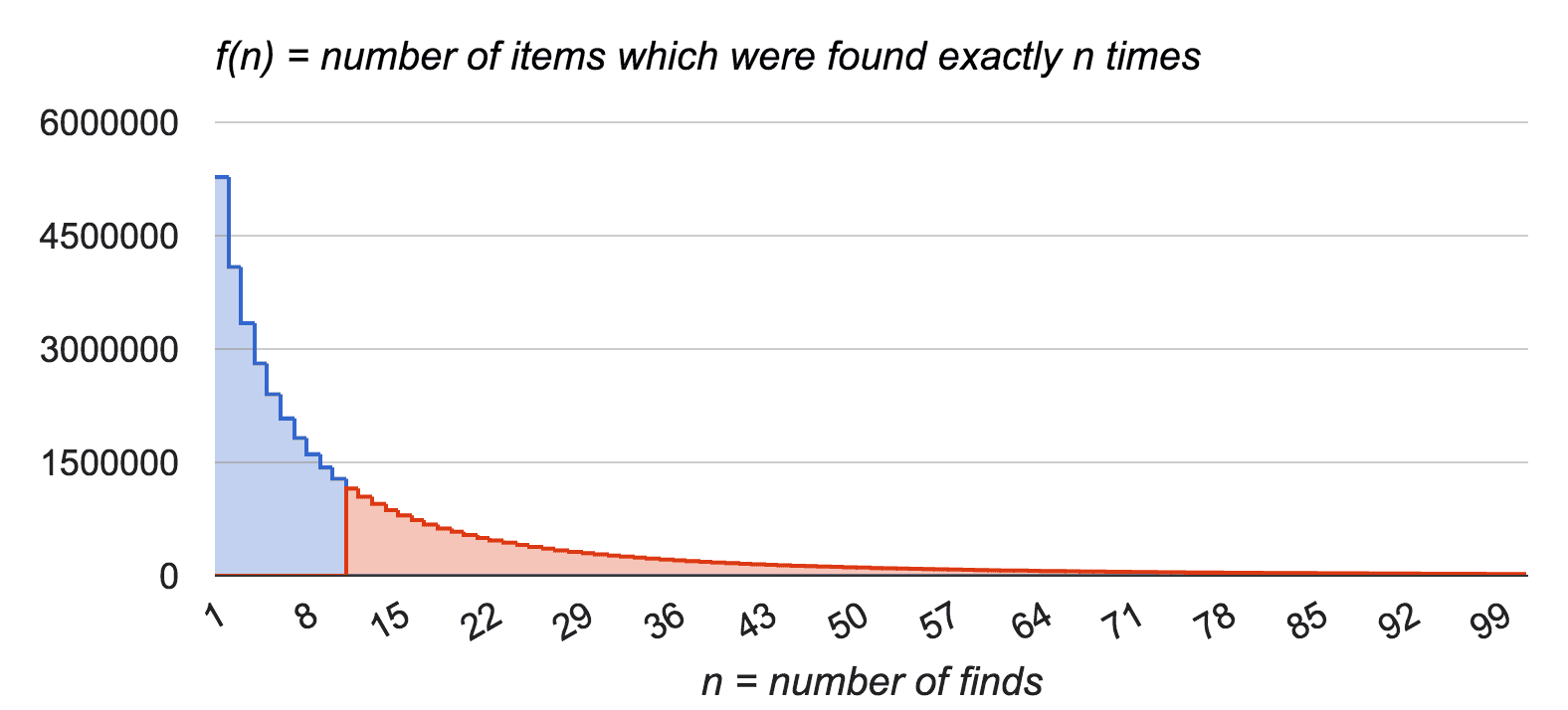
Further data analysis provided interesting facts, which are not visible in the chart:

• there are 46 millions of items found; thus some items were not requested at all;
• the standard deviation of items’ request count is pretty high, which means that some items are requested often and some of them rarely;
• the most popular item was requested 665,592 times (for better readability n is limited to 100 in the chart, but domain of f is 1 … 665,592).

Now let’s consider what happens with Cassandra requests count. We define g(n) as a number of Cassandra SELECTs generated by items which were found exactly n times. Each item found is one SELECT query sent to Cassandra — g(n) is simply f(n) * n.

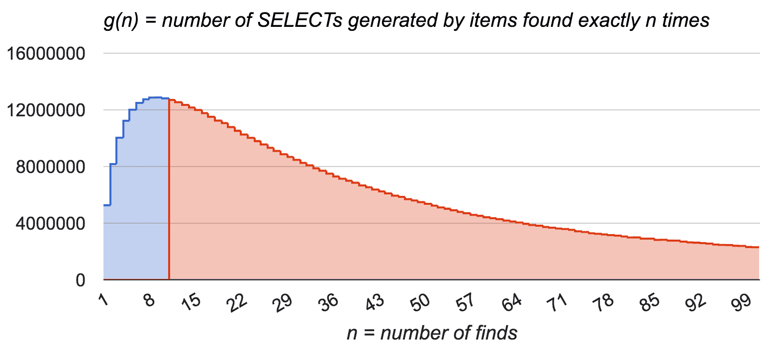
Let’s compare two charts above. Now, it’s simple to understand the cache efficiency graphically. We put vertical line on some threshold (for example, threshold 10 means that items which are requested more than 10 times in given period are cached). In the upper chart, red area is the amount of cached items, while total area is amount of all items. Similarly in the lower chart, the red part represents amount of cache hits whereas whole area is total amount of requests. As we can see, it is possible to reach high hit ratio by caching relatively small fraction of items. That proves our hyphotesis and encourages us that idea of partial items cache is worth implementing.

Computations for real-life situation

Batch computing every 24 hours doesn’t fit our case. We can’t cache items for one day because they are being updated. So we repeated computations for 15 minutes time window and with traffic limited to single service instance. We generated similar charts, but there were no straightforward conclusions from them. We decided to investigate more detailed data to extract cache hit ratio as a function of fraction of items in a cache.

We use following definitions:

• n - number of finds
• f(n) - number of items found exactly n times during a particular period
• f_all - number of all items found during a particular period (1,043,397 in our case)
• f_cached(n) = f_all - (f(1) + f(2) + … + f(n)) - number of items cached for caching threshold n
• fraction of items in a cache = f_cached(n) / f_all
• g(n) = f(n) * n - number of SELECTs generated by items found exactly n times during a particular period
• g_all - number of all SELECTs generated during a particular period (1,577,607 in our case)
• g_cached(n) = g_all - (g(1) + g(2) + … + g(n)) - number of cache hits for caching threshold n
• cache hit ratio = g_cached(n) / g_all

Here are the results for n up to 10 gathered from traffic to single node within 15 minutes:

n	f(n)	fcached(n)	fraction of items in cache	g(n)	gcached(n)	cache hit ratio
1	853589	189808	0.182	853589	724018	0.459
2	114447	75361	0.072	228894	495124	0.314
3	34329	41032	0.039	102987	392137	0.249
4	14413	26619	0.026	57652	334485	0.212
5	7287	19332	0.019	36435	298050	0.189
6	4448	14884	0.014	26688	271362	0.172
7	2957	11927	0.011	20699	250663	0.159
8	2036	9891	0.009	16288	234375	0.149
9	1491	8400	0.008	13419	220956	0.140
10	1033	7367	0.007	10330	210626	0.134

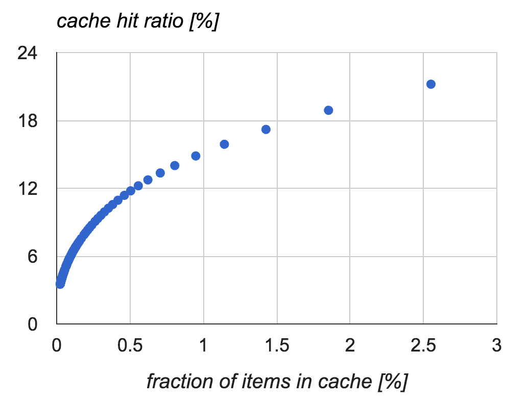
Chart generated from results (one results’ row is one blue dot in the chart) gives us clear conclusion — cache hit ratio is much higher than fraction of items in the cache.

Cache implementation

Algorithm

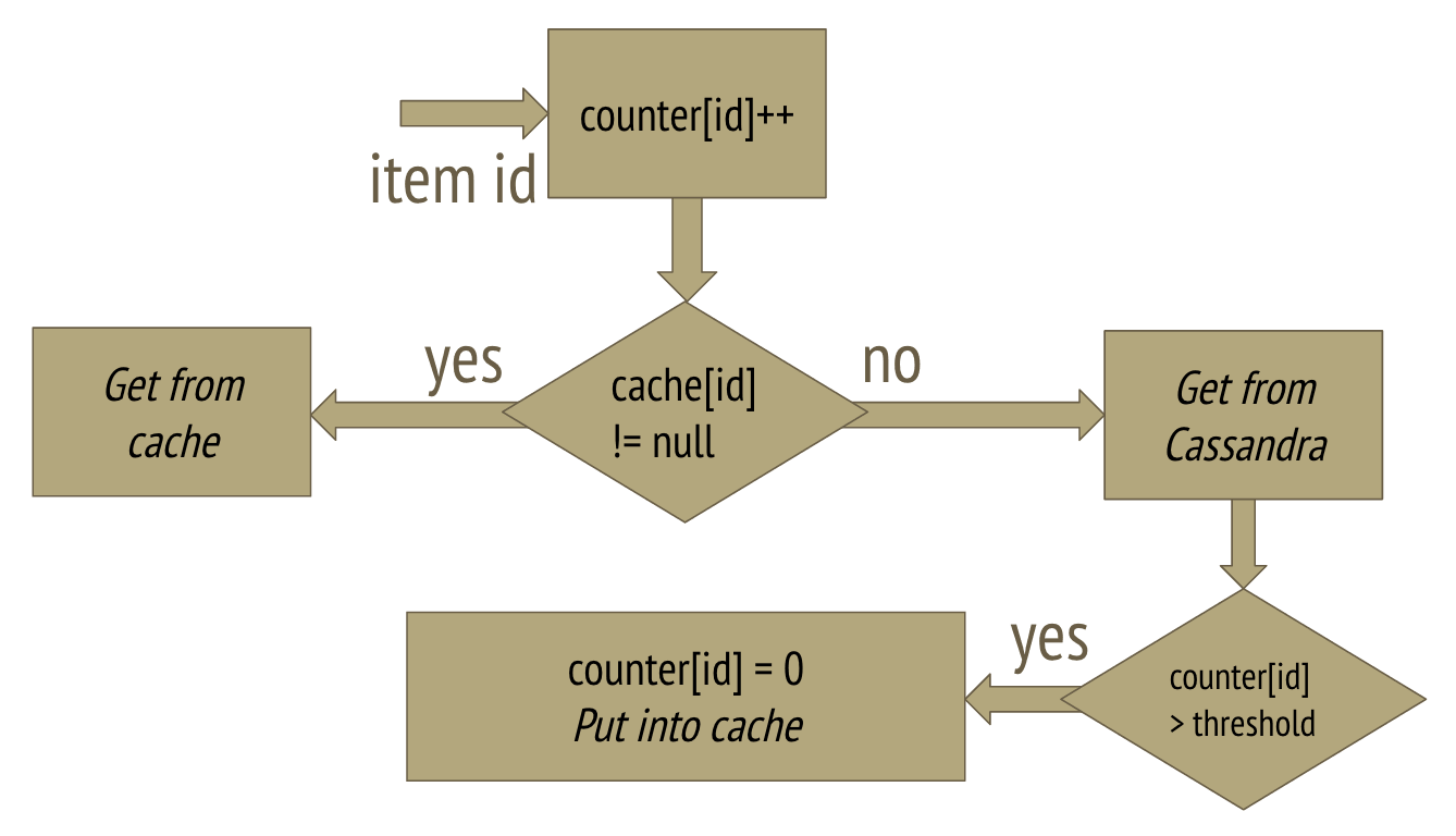
With very optimistic data, we started implementing cache in our spring-boot based application. We can describe our very simple algorithm as follows:

• We count requests for each item.
• When request for an item appears, we serve its data from cache if it is present.
• If not, data from Cassandra is loaded and if requests count for that item is above threshold, item data is cached and requests counter cleared.

The one weak point of our approach was clearing the counters. We couldn’t allow to grow counters map size infinitely. As the first approach we decided just to clear all counter when they reached given constant size. Of course this solution affects cache efficiency, but not too much — as can be observed in the charts below.

We needed two special libraries for implementing our alghoritm.

Primitives map

Our first need was primitive hash map for storing request counters. Why did we need primitive map? The memory overhead for storing 1 million of counters is at least 24 MB (at least 12 bytes extra for each Long key and 12 bytes extra for each Integer value). And we need several millions of counters.

We have read Large HashMap benchmark and gave a try to Koloboke library, which seemed to be the fastest and the most efficient large map implementation for Java.

Cache engine

The second dependency used is a cache library. We were looking for something with elegant API allowing explicit puts and gets. We did not want to utilize Spring annotations because methods in our application operate on collections, whereas cache operates on single items. We decided to check Caffeine, which provides well-known Guava Cache inspired API, but has better performance.

On production — it works!

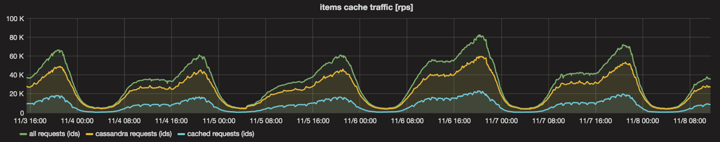
Our cache works as expected! We achieved 27% cache hit ratio in peak hours by caching only 200,000 items per service instance (remember, there are 50,000,000 items in total). We significantly decreased Cassandra cluster load and network traffic at the very small cost of 0.5 GB of RAM in each service instance.

As it was mentioned before, counter clearings slightly affected cache efficiency. After every counters clearing, items’ finds are counted starting from 0, so new items are not added to the cache for a short time. It can be observed as cyclic irregularities in the chart above.

Further improvements - get rid of counters

The counters were the weakest point of our solution. They occupied large amount of memory and cache efficiency was temporary decreased after counters clearing. We looked for a way to get rid of counters. We read about one of Caffeine features on its github project page: “size-based eviction when a maximum is exceeded based on frequency and recency”. We placed new hypothesis: “counters are unnecessary”, cache should does its job without it.

To evaluate this idea, we deployed to one production instance of our service the version without counters. Every item was being put to the cache. The cache internal logic decided itself which items should be retained and which should be removed from the cache. We compared both versions.

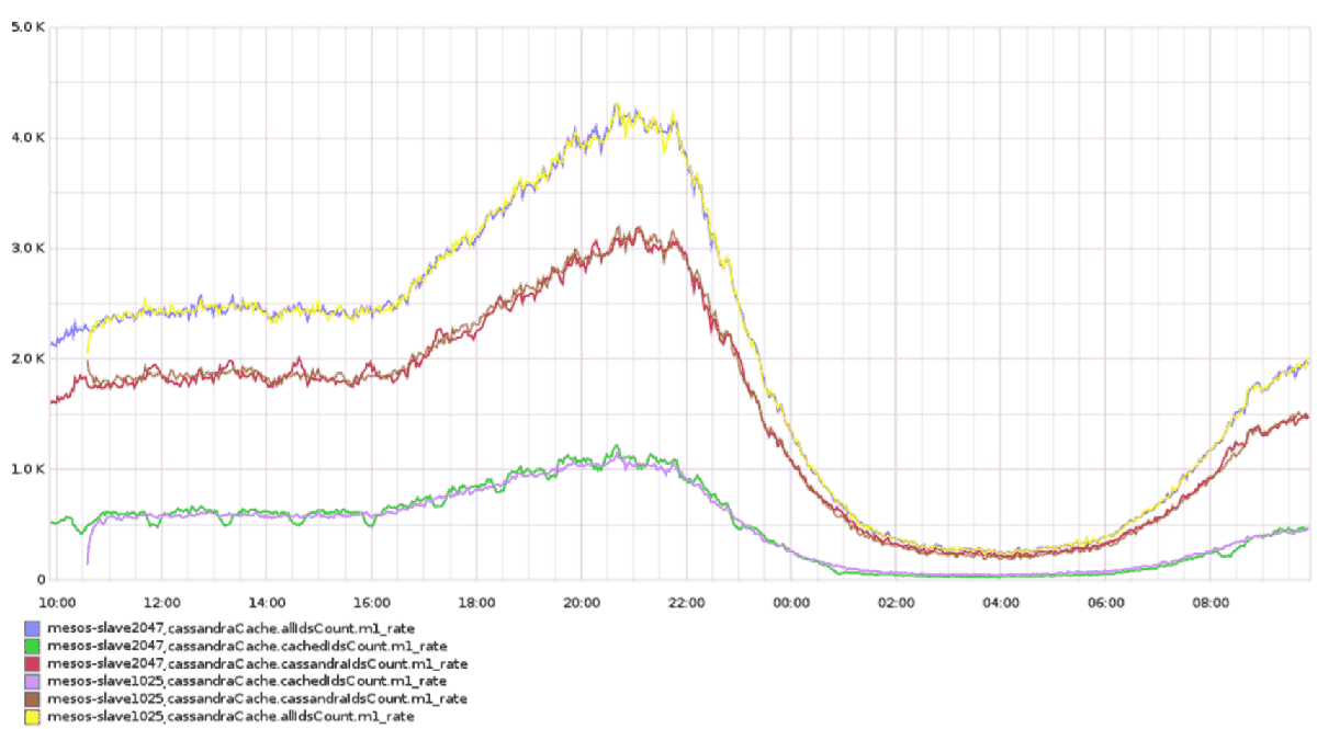
The chart above represents the rate (per second) of cached requests (cachedIdsCount.m1_rate), actual Cassandra requests (cassandraIdsCount.m1_rate) and the sum of both (allIdsCount.m1_rate). Instance mesos-slave2047 had version with counters, while mesos-slave1025 had improved version without counters. As we can see, with this improvement we simplified the algorithm, decreased memory demand and removed unwanted efficiency irregularities caused by counter clearings. Internal cache eviction logic works better than our simple counters algorithm.

What we have learned

We proved that there is no need to apply a distributed cache, as it makes the overall system architecture more complex and more difficult to maintain. Based on data, we realised that simple local cache can significantly reduce number of Cassandra queries. So our final conclusions and recommendations are:

• data characteristics is the key — know and explore your data, you can estimate cache efficiency and decide whether it is reasonable before actual implementation;
• think about how you cache — it is much more than only add @Cached annotation in a repository;
• use a cache in a way that leverages its efficiency optimization algorithms;
• consider using a cache also in non-obvious cases.